What is a calibration curve?
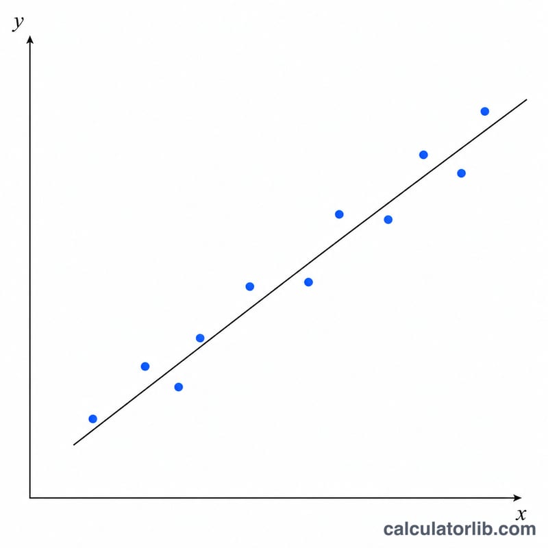
A calibration curve relates the instrument signal (absorbance, peak area, voltage, etc.) to the known concentration of a series of standards. After fitting a straight line through those standards you obtain a slope (m) and intercept (b). Once the curve is established, any measured signal from an unknown sample can be converted into a concentration. This is one of the most common workflows in analytical chemistry, spectrophotometry, chromatography, and biochemistry assays.
How to use this calculator
Enter the slope (m) and intercept (b) of your fitted calibration line, then enter the measured signal (y) of your unknown sample. The calculator solves for the concentration x. The slope and intercept come from a linear regression of your standards (signal on the y-axis, concentration on the x-axis).
The formula explained
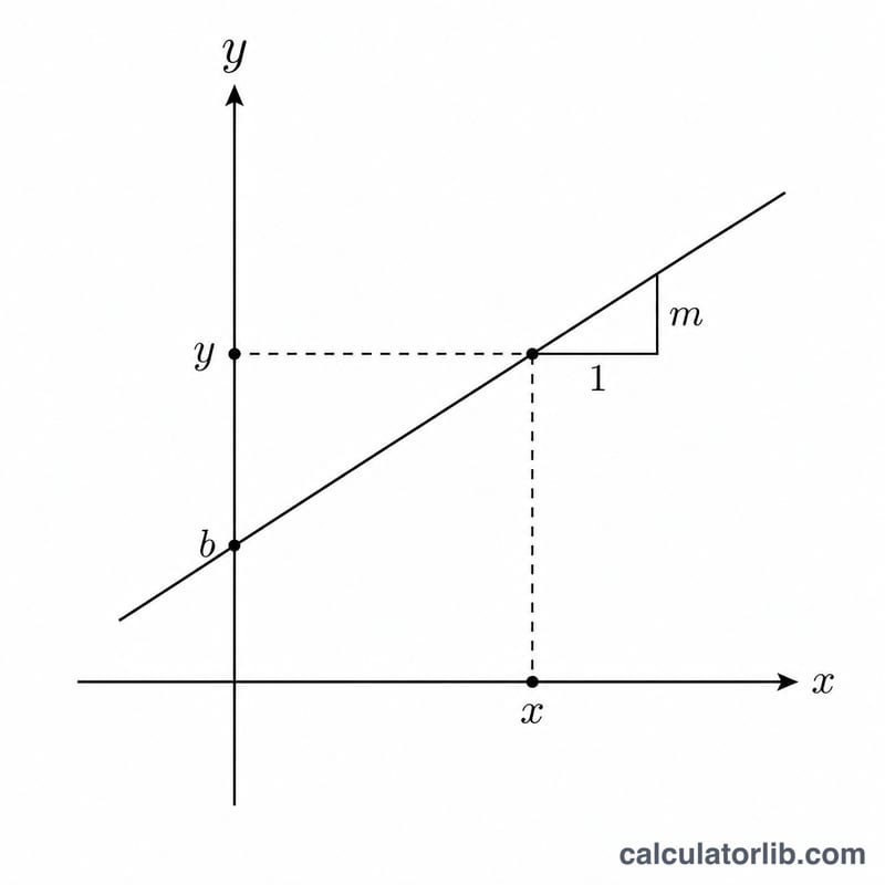
The calibration line is written as \(y = m \cdot x + b\), where y is the signal, x is the concentration, m is the slope (signal per unit concentration), and b is the intercept (the baseline signal at zero concentration). To find the concentration of an unknown, rearrange the equation to
$$x = \frac{\text{Signal }(y) - \text{Intercept }(b)}{\text{Slope }(m)}$$A larger slope means the method is more sensitive.
Worked example
Suppose a Beer–Lambert calibration gives a slope of \(m = 2.5\) absorbance units per mg/L and an intercept of \(b = 0.1\). A sample reads an absorbance of \(y = 5.1\). Then
$$x = \frac{5.1 - 0.1}{2.5} = \frac{5.0}{2.5} = \textbf{2.0 mg/L}$$More Worked Examples
Each example uses the calibration equation \(y = mx + b\) rearranged to solve for concentration: \(x = \dfrac{y - b}{m}\). The slope \(m\) and intercept \(b\) come from your standard curve; \(y\) is the measured signal of the unknown.
Example 1 — HPLC peak area (µM)
A chromatography calibration gives slope \(m = 1500\) (peak-area units per µM) and intercept \(b = 250\). An unknown sample produces a peak area of \(y = 9250\).
$$x = \frac{9250 - 250}{1500} = \frac{9000}{1500} = 6\ \mu M$$The unknown concentration is 6 µM.
Example 2 — Fluorescence curve with negative intercept
A fluorescence assay yields a slightly negative intercept from blank correction: \(m = 0.045\) RFU per ng/mL and \(b = -0.012\) RFU. The sample reads \(y = 0.528\) RFU.
$$x = \frac{0.528 - (-0.012)}{0.045} = \frac{0.540}{0.045} = 12\ \text{ng/mL}$$The result is 12 ng/mL. A negative intercept is common after blank subtraction and simply shifts the line down slightly.
Example 3 — Signal below intercept (below detection)
A UV-Vis curve has \(m = 0.080\) AU per mg/L and \(b = 0.020\) AU. A very dilute sample reads \(y = 0.012\) AU, which is below the intercept.
$$x = \frac{0.012 - 0.020}{0.080} = \frac{-0.008}{0.080} = -0.1\ \text{mg/L}$$The math gives -0.1 mg/L. A negative concentration is not physically meaningful — it indicates the analyte is effectively absent or below the limit of detection. Report it as < LOD rather than a negative value.
How Slope and Intercept Affect the Result
The slope \(m\) reflects the method's sensitivity — a steeper line means a larger signal change per unit concentration, so the same signal corresponds to a lower concentration. The intercept \(b\) shifts the line vertically; raising it reduces the computed concentration for a fixed signal. The table below holds the measured signal constant at \(y = 1.00\) and varies \(m\) and \(b\).
| Slope \(m\) | Intercept \(b\) | Signal \(y\) | Concentration \(x = (y-b)/m\) |
|---|---|---|---|
| 0.10 | 0.00 | 1.00 | 10.0 |
| 0.20 | 0.00 | 1.00 | 5.0 |
| 0.50 | 0.00 | 1.00 | 2.0 |
| 0.20 | 0.10 | 1.00 | 4.5 |
| 0.20 | 0.20 | 1.00 | 4.0 |
| 0.20 | -0.10 | 1.00 | 5.5 |
Reading down the first three rows: doubling the slope halves the concentration for the same signal — higher sensitivity packs more signal into less analyte. Comparing the rows where \(m = 0.20\): increasing the intercept lowers the result, while a negative intercept raises it. Always use the actual fitted slope and intercept from your own standards rather than assuming a value.
Interpreting Your Concentration Result
- Stay within the calibrated range. The linear equation is only validated between your lowest and highest standards. Concentrations computed from signals outside that range are extrapolations and may be inaccurate because the response often becomes non-linear at high or low extremes.
- Dilute high signals. If a sample's signal exceeds the highest standard, dilute it by a known factor, re-measure within range, then multiply the computed concentration by that dilution factor.
- Near or below the intercept approaches the limit of detection. As the measured signal approaches \(b\), the computed concentration approaches zero, and signals below \(b\) yield negative (non-physical) values. These should be reported as below the limit of detection (< LOD) rather than as exact numbers.
- Check R² and linearity. A high coefficient of determination (commonly \(R^2 \ge 0.995\) for quantitative work) supports the assumption that the relationship is linear. A poor fit means the slope and intercept — and therefore every computed concentration — carry large uncertainty. Inspect a residual plot, not just R², to confirm the model is appropriate.
- Units are inherited from the standards. The concentration is reported in whatever units your calibration standards used (µM, ng/mL, mg/L, etc.). The slope already carries the signal-per-concentration units, so the result automatically matches the standards.
- Replicates and propagation. Averaging replicate signal measurements reduces random error in \(y\), which directly improves the precision of the computed \(x\). Uncertainty in the slope and intercept from the regression also propagates into the final concentration.
This is general analytical guidance; follow your laboratory's validated method and quality-control criteria for reporting decisions.
FAQ
What units does x have? Whatever concentration units you used for your standards (mg/L, µM, ppm, etc.).
What if the intercept is negative? That is fine — just enter it as a negative number; the formula handles it.
Can the slope be zero? No useful calibration has a zero slope; if you enter 0 the result defaults to 0 to avoid dividing by zero.