
What this calculator does
This tool numerically solves a first-order ordinary differential equation of the form \(y' = F(x, y)\) with a given initial condition \(y(x_0) = y_0\), over the interval from \(x_0\) to \(x_n\). It uses the classical fourth-order Runge-Kutta method (RK4), one of the most widely used and reliable single-step integrators in numerical analysis. The result is a table of points \((x_i, y_i)\) approximating the true solution, plus the final value \(y(x_n)\). This is a pure-math tool with no country or unit scope.
How to use it
Enter the right-hand side \(F(x,y)\) as an expression in x and y (for example 1-y^2, x+y, x*y, or sin(x)+y). Supported operators are + - * / ^ and functions such as sin, cos, tan, exp, log, ln, sqrt, abs, tanh, plus constants pi and e. Set the start \(x_0\), initial value \(y_0\), end \(x_n\), and choose how many equal subdivisions \(n\) to use. More subdivisions give higher accuracy because the global error of RK4 shrinks like \(h^4\).
The formula explained
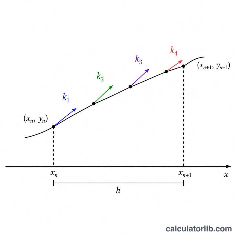
The interval is split into \(n\) equal steps of width \(h = (x_n - x_0)/n\). At each step RK4 samples the slope four times: once at the start (\(k_1\)), twice at the midpoint (\(k_2\), \(k_3\)), and once at the end (\(k_4\)). The next value is a weighted average,
$$y_{n+1} = y_n + \frac{1}{6}\left(k_1 + 2k_2 + 2k_3 + k_4\right)$$This cancels error terms up to fourth order, giving a local truncation error of \(O(h^5)\) and global error \(O(h^4)\).
Worked example
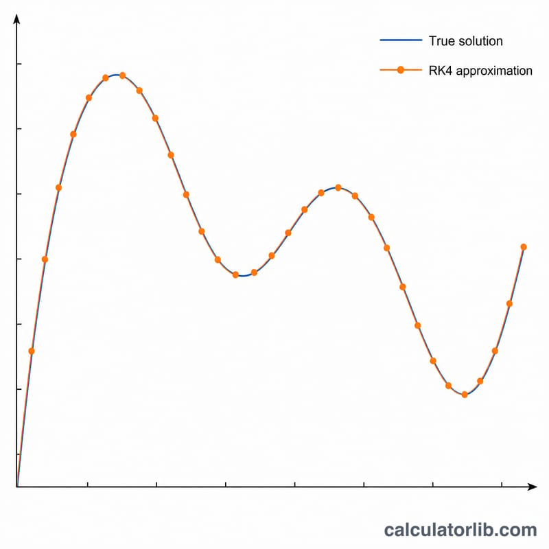
Solve \(y' = 1 - y^2\) with \(x_0 = 0\), \(y_0 = 0\), \(x_n = 1\) and \(n = 10\) (\(h = 0.1\)). The exact solution is \(y = \tanh(x)\). The first RK4 step gives
$$y_1 = 0.0996679,\quad \tanh(0.1) = 0.0996680$$After all ten steps,
$$y(1) = 0.7615942,\quad \tanh(1) = 0.7615942$$to seven digits.
FAQ
Why is RK4 better than Euler's method? Euler uses one slope per step (error \(O(h)\)). RK4 uses four and averages them, achieving \(O(h^4)\) accuracy for the same step size, so far fewer steps are needed for a target precision.
How many steps should I pick? Start with 50. If the solution is smooth, that is usually plenty; for rapidly varying or near-stiff problems, increase to 100, 200 or 500.
What if I get NaN or Infinity? The solution may have diverged or \(F(x,y)\) hit an invalid operation (like log of a negative or division by zero). Check the expression and try a smaller interval or more steps.