Connect via MCP →

Enter Calculation

Formula

Advertisement

Results

Approximate y at the final x = 1
0.135296935
y' (= p) at that point: -0.1351841876
Method 2nd-order Runge-Kutta (midpoint), local error O(h^3)
Step size h 0.02
Number of steps n 50
x y y' = p
0.0000000000000000 0.0000000000000000 1.0000000000000000
0.020000000000000000 0.019200000000000000 0.92240000000000000
0.040000000000000000 0.036894720000000000 0.84934720000000000
0.060000000000000000 0.053172670463999996 0.78060434278399990
0.080000000000000000 0.068117735709081600 0.71594578469232630
0.10000000000000000 0.081809400586607000 0.65515694969774430
0.12000000000000001 0.094322966500334410 0.59803380843614800
0.14000000000000000 0.10572975724910819 0.54438238107427720
0.16000000000000000 0.11609731515993502 0.49401826294618173
0.18000000000000000 0.12548958795637377 0.44676617193727500
0.19999999999999998 0.13396710678720436 0.40245951663989300
0.21999999999999997 0.14158715582126055 0.36093998434738000
0.23999999999999996 0.14840393379607325 0.32205714799495050
0.25999999999999995 0.15446870789053943 0.28566809119500390
0.27999999999999997 0.15982996027517107 0.25163705055227820
0.30000000000000000 0.16453352767755470 0.21983507448028827
0.32000000000000000 0.16862273428543417 0.19013969777498171
0.34000000000000000 0.17213851829528548 0.16243463123452180
0.36000000000000004 0.17511955240035207 0.13660946564564497
0.38000000000000006 0.17760235849882816 0.11255938948719588
0.40000000000000010 0.17962141689018327 0.090184919730279480
0.42000000000000010 0.18120927021549250 0.069391645142043710
0.44000000000000010 0.18239662238604734 0.050089981526471296
0.46000000000000013 0.18321243273344676 0.032194938360768685
0.48000000000000015 0.18368400560378675 0.015625896310044324
0.50000000000000010 0.18383707560845658 0.00030639512601406127
0.52000000000000010 0.18369588873438927 -0.013836068542494098
0.54000000000000010 0.18328327950738588 -0.026870233878397654
0.56000000000000020 0.18262074439331474 -0.038861259595601230
0.58000000000000020 0.18172851161356454 -0.049870899020389145
0.60000000000000020 0.18062560754308220 -0.059957666948328710
0.62000000000000020 0.17932991985163985 -0.069176998652447110
0.64000000000000020 0.17785825754163154 -0.077581401401623160
0.66000000000000030 0.17622640802868705 -0.085220598832054500
0.68000000000000030 0.17444919140468865 -0.092141668499290240
0.70000000000000030 0.17254051201637852 -0.098389172923625410
0.72000000000000030 0.17051340748663180 -0.10400528442760995
0.74000000000000030 0.16838009529963238 -0.10902990405100074
0.76000000000000030 0.16615201706561347 -0.11350077481565485
0.78000000000000040 0.16383988057550042 -0.11745358960059915
0.80000000000000040 0.16145369975070850 -0.12092209387579109
0.82000000000000040 0.15900283258849274 -0.12393818353188411
0.84000000000000040 0.15649601719860975 -0.12653199803260615
0.86000000000000040 0.15394140602262482 -0.12873200910612914
0.88000000000000040 0.15134659832296904 -0.13056510518203110
0.90000000000000050 0.14871867102481567 -0.13205667177110950
0.92000000000000050 0.14606420798999050 -0.13323066797637725
0.94000000000000050 0.14338932779845207 -0.13410969931504166
0.96000000000000050 0.14069971010936450 -0.13471508702311555
0.98000000000000050 0.13800062067043317 -0.13506693400652098
1.0000000000000004 0.13529693504097162 -0.13518418759510423

What this calculator does

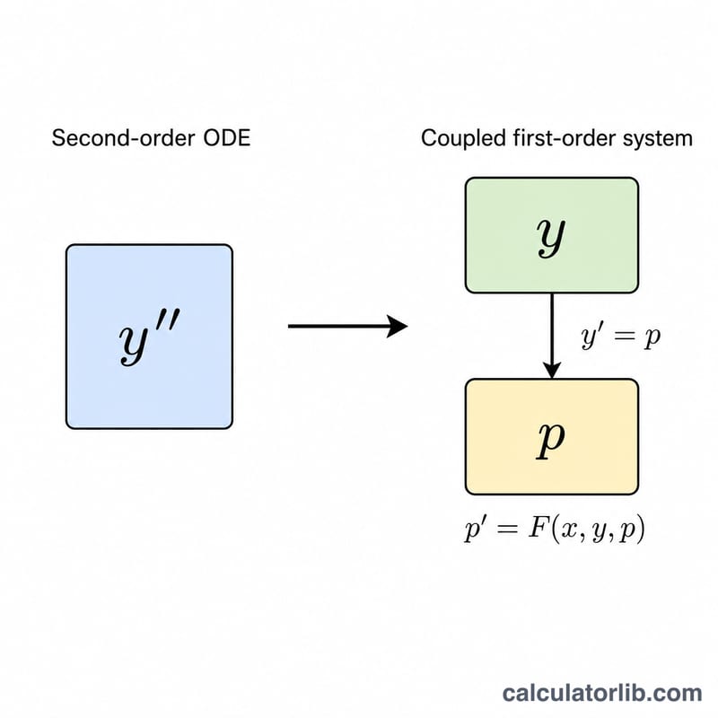
This tool numerically solves a second-order ordinary differential equation written in the form \(y'' = F(x, y, y')\) over an interval [x0, xn], using the second-order Runge-Kutta method (the midpoint/modified-Euler RK2 scheme). You provide the right-hand side F as an expression in x, y and p (where p stands for y'), the initial values y(x0) and y'(x0), the interval endpoints and the number of steps. The result is a table of (x, y, y') values marching across the interval. This is pure numerical analysis, so it applies identically anywhere.

How to use it

Type the forcing function F using x, y and p, for example -4*p-4*y for \(y'' = -4y' - 4y\). Operators + - * / ^ (or **) and functions sin, cos, tan, exp, log, ln, sqrt, abs, pow plus constants pi, e are supported. Set x0, the initial y0 and y'0 = p0, the end point xn, and pick the number of subintervals n. More steps means a smaller step size \(h = (x_n - x_0)/n\) and lower error (global error is \(O(h^2)\)).

The formula explained

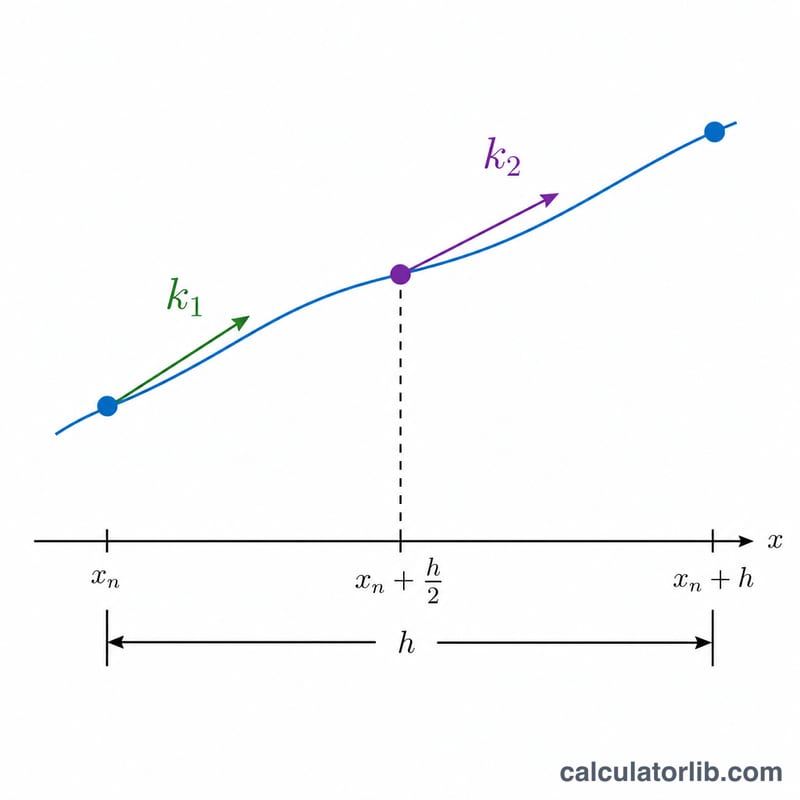
The equation is first reduced to a first-order system by letting \(p = y'\), giving \(y' = p\) and \(p' = F(x, y, p)\). Each RK2 step samples the slope at the start and at the midpoint and combines them: \(j_1 = h\cdot F(x,y,p)\), \(k_1 = h\cdot p\), then \(j_2\) and \(k_2\) are evaluated at the midpoint and used to advance p and y. The local truncation error is \(O(h^3)\) per step.

Advertisement
Schematic of reducing a second-order ODE to two coupled first-order equations
A second-order ODE is rewritten as two coupled first-order equations using \(y' = p\).
Diagram showing the RK2 midpoint method estimating a slope at the midpoint of a step
The midpoint RK2 method evaluates an initial slope, then uses the slope at the interval midpoint to advance the solution.

Worked example

With F = -4*p-4*y, x0 = 0, y0 = 0, p0 = 1, xn = 1, n = 50, the step size is \(h = 0.02\). The first step gives \(y_1 = 0.0192\) and \(p_1 = 0.9224\). Iterating to x = 1 yields $$y(1) \approx 0.13533 \quad\text{and}\quad y'(1) \approx -0.13533,$$ matching the exact solution \(y = x\cdot e^{-2x}\) whose value at x = 1 is \(e^{-2} = 0.135335\).

FAQ

Is this RK2 or RK4? This is second-order Runge-Kutta (midpoint rule), not the classical fourth-order method, so it is only second-order accurate globally.

Can xn be less than x0? Yes. The step size simply becomes negative and integration proceeds backward, which is mathematically valid.

Why did I get an error row? Evaluation problems such as division by zero, log of a non-positive number or sqrt of a negative number inside F stop the integration and report the location.

Last updated: