Connect via MCP →

Enter Calculation

Formula

Advertisement

Results

Approximate y at x = 1
0.761577877980713414
y_n = f(xn) via 2nd-order Runge-Kutta (midpoint)
Step size h = (xn - x0)/n 0.02
Number of subdivisions n 50
i x_i y_i
0 0 0
1 0.0200000000000000004 0.0199980000000000019
2 0.0400000000000000008 0.0399800071983202471
3 0.0599999999999999978 0.0599300791260564958
4 0.0800000000000000017 0.0798323752456768093
5 0.100000000000000006 0.0996712070597656069
6 0.119999999999999996 0.119431087194065227
7 0.140000000000000013 0.139096777131368088
8 0.160000000000000003 0.158653333288278714
9 0.179999999999999993 0.178086151145683907
10 0.200000000000000011 0.197381007165616462
11 0.220000000000000001 0.216524098251703712
12 0.239999999999999991 0.235502078537144943
13 0.260000000000000009 0.254302093312726574
14 0.280000000000000027 0.272911809937302630
15 0.299999999999999989 0.291319445603977822
16 0.320000000000000007 0.309513791866466770
17 0.340000000000000024 0.327484235861315365
18 0.359999999999999987 0.345220778192424416
19 0.380000000000000004 0.362714047474209156
20 0.400000000000000022 0.379955311558386910
21 0.419999999999999984 0.396936485496481195
22 0.440000000000000002 0.413650136315375394
23 0.460000000000000020 0.430089484706401570
24 0.479999999999999982 0.446248403749321843
25 0.5 0.462121414811006104
26 0.520000000000000018 0.477703680774537398
27 0.540000000000000036 0.492990996767839251
28 0.560000000000000053 0.507979778571714169
29 0.579999999999999960 0.522667048895444131
30 0.599999999999999978 0.537050421713912929
31 0.619999999999999996 0.551128084863663603
32 0.640000000000000013 0.564898781096544900
33 0.660000000000000031 0.578361787788779114
34 0.680000000000000049 0.591516895500573292
35 0.700000000000000067 0.604364385576987795
36 0.719999999999999973 0.616905006974859837
37 0.739999999999999991 0.629139952493357413
38 0.760000000000000009 0.641070834577409543
39 0.780000000000000027 0.652699660854015540
40 0.800000000000000044 0.664028809551470589
41 0.820000000000000062 0.675061004941040266
42 0.839999999999999969 0.685799292929734738
43 0.859999999999999987 0.696247016921744177
44 0.880000000000000004 0.706407794054930038
45 0.900000000000000022 0.716285491907665772
46 0.920000000000000040 0.725884205760389145
47 0.940000000000000058 0.735208236485572653
48 0.959999999999999964 0.744262069129523307
49 0.979999999999999982 0.753050352239556631
50 1 0.761577877980713414

What is the Runge-Kutta 2nd Order Method Calculator?

This tool numerically solves a first-order ordinary differential equation (ODE) of the form \(y' = F(x, y)\) over an interval \([x_0, x_n]\), starting from the initial condition \(y_0 = f(x_0)\). It uses the 2nd-order Runge-Kutta method (the midpoint method), producing a table of \((x, y)\) approximations and the final value \(y_n = f(x_n)\). It is a universal mathematical tool with no country or jurisdiction restrictions.

How to use it

Enter the right-hand side \(F(x,y)\) as a math expression in \(x\) and \(y\) (for example 1-y^2, x*y, or sin(x)+y). Provide the initial point \(x_0\) and \(y_0\), the end of the range \(x_n\), and choose the number of equal subdivisions \(n\). The interval is split into \(n\) steps of size \(h = (x_n - x_0)/n\). A larger \(n\) gives a finer step and better accuracy. The display-precision selector only controls how many significant digits are shown.

The formula explained

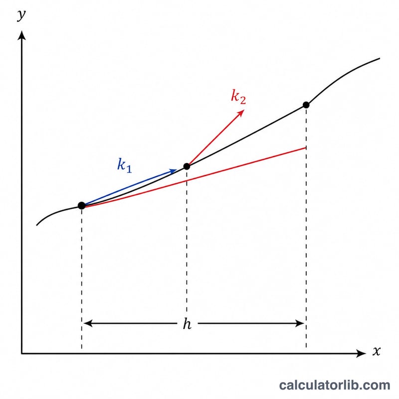
The midpoint Runge-Kutta scheme advances the solution one step at a time:

$$k_1 = h \cdot F(x_i, y_i)$$$$k_2 = h \cdot F\left(x_i + \frac{h}{2},\; y_i + \frac{k_1}{2}\right)$$$$y_{i+1} = y_i + k_2, \qquad x_{i+1} = x_i + h$$

The slope is estimated at the midpoint of the step, which cancels the leading error term. The local truncation error is \(O(h^3)\) and the global error is \(O(h^2)\), so halving \(h\) roughly quarters the error.

Advertisement
Diagram showing midpoint slope estimate used to advance one RK2 step along a solution curve
The midpoint method uses slope \(k_1\) to find a midpoint, then uses the midpoint slope \(k_2\) to take the full step.

Worked example

Solve \(y' = 1 - y^2\) with \(x_0 = 0\), \(y_0 = 0\), \(x_n = 1\), \(n = 50\) (so \(h = 0.02\)). The exact solution is \(y = \tanh(x)\). Step 1: \(k_1 = 0.02 \cdot (1-0) = 0.02\); \(k_2 = 0.02 \cdot (1-0.01^2) = 0.019998\); \(y_1 = 0.019998\). Continuing all 50 steps gives \(y(1) \approx 0.76159\), matching \(\tanh(1) \approx 0.7615942\) to five decimals.

FAQ

How accurate is it? Accuracy improves with larger \(n\) because global error scales as \(h^2\). For stiff equations or very large steps the result can diverge.

Can \(x_n\) be less than \(x_0\)? Yes. Then \(h\) is negative and the method integrates backward in \(x\), which is still valid.

What functions can I use? Standard ones: sin, cos, tan, exp, ln, log, sqrt, plus +, -, *, /, ^ and parentheses, and the constants e and pi.

Last updated: