What is exponential regression?
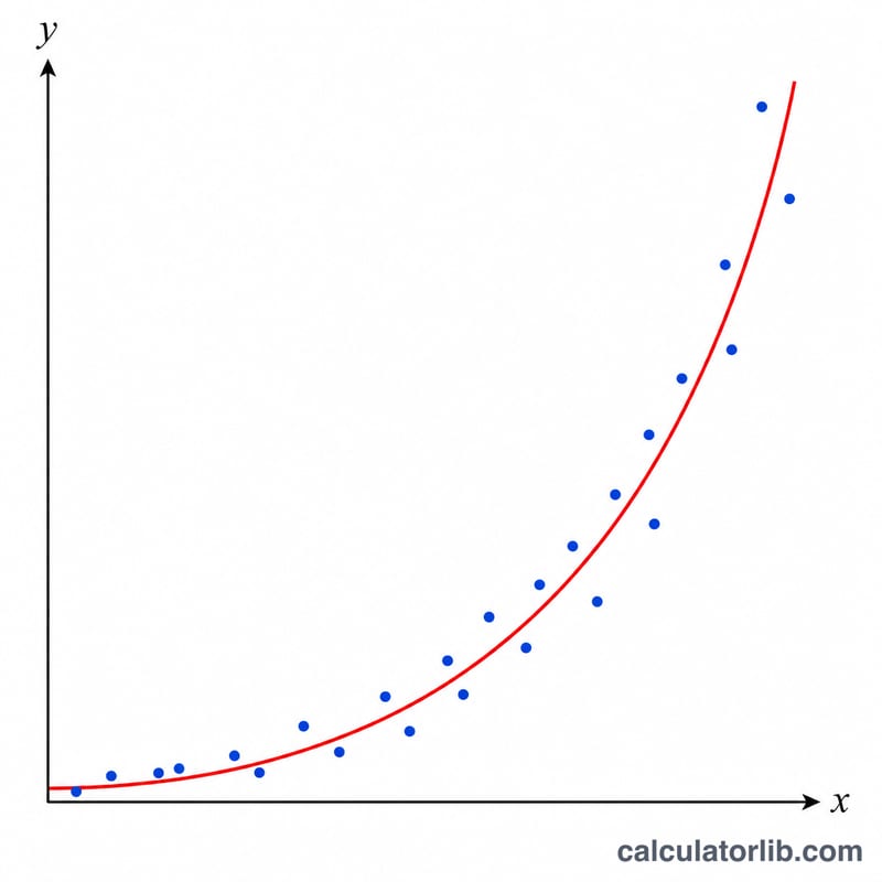
Exponential regression fits a curve of the form \(y = A \cdot B^{x}\) to a set of paired observations. It is the right tool whenever a quantity grows or decays by a roughly constant factor for each unit increase in x — population growth, compound interest, radioactive decay, bacterial cultures and many natural processes. This is a universal statistical tool with no region-specific rules.
How to use it
Enter your data one pair per line as x,y. You need at least two points, the x values must not all be identical, and every y value must be strictly positive (the method takes the natural logarithm of y). Pick the number of display digits, then read off A, B and the correlation coefficient r.
The formula explained
The model is non-linear, but taking logarithms makes it linear: \(\ln(y) = \ln(A) + x \cdot \ln(B)\). We therefore run an ordinary least-squares line fit on the transformed points \((x_i, \ln y_i)\). With \(\bar{x}\) the mean of x and meanLnY the mean of ln y, define $$S_{xx} = \sum (x_i - \bar{x})^2, \quad S_{yy} = \sum (\ln y_i - \text{meanLnY})^2, \quad S_{xy} = \sum (x_i - \bar{x})(\ln y_i - \text{meanLnY}).$$ Then $$B = \exp\!\left(\frac{S_{xy}}{S_{xx}}\right), \quad A = \exp(\text{meanLnY} - \bar{x} \cdot \ln B), \quad r = \frac{S_{xy}}{\sqrt{S_{xx}} \cdot \sqrt{S_{yy}}}.$$
Worked example
For the points (1, 2.7), (2, 7.4), (3, 20.1), (4, 54.6), (5, 148.4): \(n = 5\), \(\bar{x} = 3\), \(\text{meanLnY} \approx 2.99906\). \(S_{xx} = 10\), \(S_{xy} \approx 10.01167\), \(S_{yy} \approx 10.02337\). So $$B = \exp(1.001167) \approx 2.7215, \quad A = \exp(2.99906 - 3 \cdot 1.001167) \approx 0.9956, \quad r \approx 0.99999985.$$ The fitted model \(y \approx 0.9956 \cdot 2.7215^{x}\) closely matches the underlying \(y \approx e^{x}\).
Interpreting Your Result
An exponential regression returns three numbers — \(A\), \(B\) and \(r\) — that together describe the model \(y = A \cdot B^{\,x}\). Here is how to read each one.
The base \(B\): growth or decay
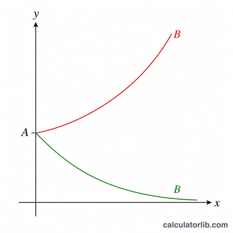
The base \(B\) controls the direction and speed of change for every one-unit increase in \(x\):
- \(B > 1\) means growth. Each step in \(x\) multiplies \(y\) by \(B\), so the curve rises. The per-unit percentage change is \((B-1)\times100\%\). For example, \(B = 1.08\) corresponds to 8% growth per unit of \(x\).
- \(B < 1\) means decay. Each step multiplies \(y\) by less than one, so the curve falls toward zero. The same formula \((B-1)\times100\%\) gives a negative result; e.g. \(B = 0.85\) is a \(-15\%\) change per unit.
- \(B = 1\) is flat. \(y\) stays equal to \(A\) regardless of \(x\) (zero percent change).
The coefficient \(A\): the y-intercept
\(A\) is the value of \(y\) when \(x = 0\), because \(A \cdot B^{0} = A\). It anchors the curve vertically and represents the starting amount, the initial population, the principal, or the dose at the origin of your \(x\)-axis.
The correlation coefficient \(r\): fit on the log scale
This fit works by taking \(z_i = \ln y_i\) and running an ordinary linear regression of \(z\) against \(x\). Consequently, \(r\) measures how well the log-transformed data \(\ln(y)\) fall on a straight line — not how well the raw \(y\) values fit the curve. A value of \(r\) close to \(+1\) or \(-1\) indicates a strong exponential relationship; the sign matches the direction (positive for growth, negative for decay).
Using standard correlation interpretation bands for \(|r|\):
- 0.9 – 1.0: very strong fit — the data closely follow the exponential model.
- 0.7 – 0.9: strong fit — exponential is a good description with some scatter.
- 0.5 – 0.7: moderate fit — a trend exists but other factors are at play.
- below 0.5: weak fit — an exponential model may not be appropriate.
Because \(r\) reflects the log-scale fit, a high \(r\) does not guarantee small errors on the original \(y\) scale; large \(y\) values are weighted less after the \(\ln\) transform. Always plot the fitted curve against your raw data as a sanity check.
FAQ
Why must y be positive? The fit works on \(\ln(y)\), and the logarithm of zero or a negative number is undefined.
What does r mean here? It is the correlation between x and ln(y). Use the guide: \(0.7 < |r| \le 1\) strong, \(0.4 < |r| < 0.7\) moderate, \(0.2 < |r| < 0.4\) weak, below 0.2 none.
What if all my x values are the same? Then \(S_{xx} = 0\) and the slope is undefined; supply at least two distinct x values.


