What this calculator does
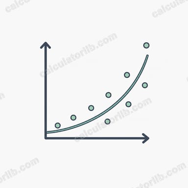
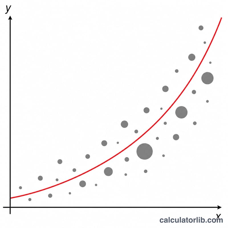
This tool fits an ab-exponential trend line of the form \(y = A\cdot B^{x}\) to a frequency distribution table of data points. Each row carries an x value, a y value, and a frequency f (the number of times, or weight, that the (x, y) pair occurs). It is a pure statistical method and applies identically everywhere — no units, no jurisdiction.
How to use it
Enter one data point per line as x, y, f. The y value must be strictly positive because the method takes the natural logarithm of y. If you want an ordinary unweighted fit, set every frequency to 1 (you may also omit the third number, in which case f = 1 is assumed). Choose the number of significant figures for the displayed coefficients, then read off A, B and the correlation coefficient r.
The formula explained
The trick is to linearize the model: taking logs of \(y = A\cdot B^{x}\) gives \(\ln y = \ln A + x\cdot\ln B\), a straight line in (x, ln y) space. We run a frequency-weighted least-squares regression of ln y on x. With \(n = \sum f\), weighted means \(\bar{x}\) and \(\overline{\ln y}\), and weighted sums \(S_{xx}\), \(S_{yy}\), \(S_{xy}\), the slope is \(S_{xy}/S_{xx}\) and the intercept is \(\overline{\ln y} - \bar{x}\cdot\text{slope}\). Exponentiating gives \(B = e^{\text{slope}}\) and \(A = e^{\text{intercept}}\). The correlation coefficient \(r = S_{xy} / (\sqrt{S_{xx}} \cdot \sqrt{S_{yy}})\) measures how well the log-linear model fits.
$$\begin{gathered} y = A \cdot B^{x}, \qquad B = e^{\,S_{xy}/S_{xx}}, \quad A = e^{\,\overline{\ln y} - \bar{x}\,(S_{xy}/S_{xx})} \\[1.5em] \text{where}\quad \left\{ \begin{aligned} n &= \textstyle\sum f, \quad \bar{x} = \frac{\sum f x}{n}, \quad \overline{\ln y} = \frac{\sum f \ln y}{n} \\ S_{xx} &= \textstyle\sum f x^{2} - n\,\bar{x}^{2} \\ S_{xy} &= \textstyle\sum f\,x \ln y - n\,\bar{x}\,\overline{\ln y} \\ x,\,y,\,f &= \text{Data points (x, y, f)} \end{aligned} \right. \end{gathered}$$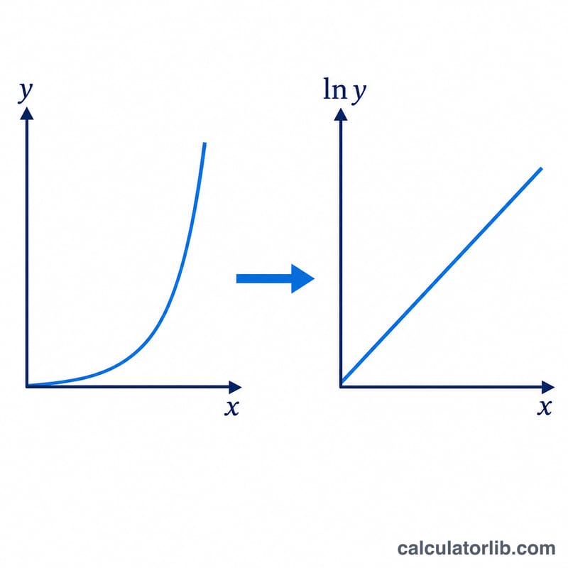
Worked example
For the perfectly doubling data (1, 2), (2, 4), (3, 8), (4, 16) all with f = 1: \(n = 4\), \(\bar{x} = 2.5\), \(\overline{\ln y} = 1.732868\), \(S_{xx} = 5\), \(S_{xy} = 3.465735\), \(S_{yy} = 2.402224\). Then $$B = e^{3.465735/5} = e^{0.693147} = 2,$$ \(A = e^{0} = 1\), and \(r = 1\). So the fitted curve is \(y = 1\cdot 2^{x}\), exactly as expected.
FAQ
What does the frequency column do? It weights each data point by how often it occurs, so a row with f = 5 counts the same as five identical rows. Use f = 1 everywhere for a normal regression.
How do I read r? \(|r| > 0.7\) indicates a strong correlation, 0.4–0.7 moderate, 0.2–0.4 weak, and below 0.2 essentially none. r is computed in (x, ln y) space.
Why must y be positive? The model takes the natural log of y; ln y is undefined for \(y \le 0\), so non-positive rows are ignored.


