What is exponential regression?
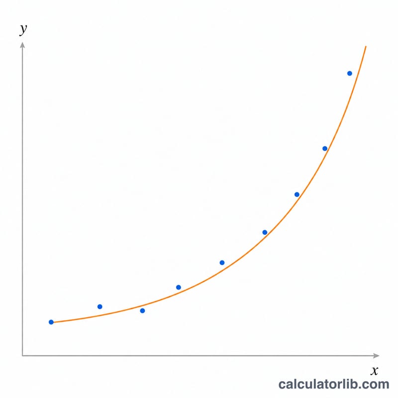
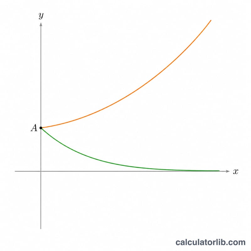
Exponential regression fits a curve of the form \(y = A\cdot e^{Bx}\) to a set of paired data points. It is the standard tool for modeling quantities that grow or decay at a rate proportional to their current size, such as population growth, radioactive decay, compound interest, or bacterial cultures. This calculator is a pure mathematical and statistical tool, so it applies identically everywhere with no country-specific assumptions.
How to use it
Enter your independent values in the X values box and your dependent values in the Y values box, both as comma-separated numbers. The two lists must have the same number of entries, you need at least two points, and every Y value must be strictly positive (the method requires the natural logarithm of y). Choose the display precision, then read off the fitted coefficients A and B, the correlation coefficient r, and the assembled equation.
The formula explained
Because \(y = A\cdot e^{Bx}\) is non-linear, we linearize it by taking natural logarithms: \(\ln y = \ln A + B\cdot x\). This is an ordinary linear regression of \(\ln(y)\) against \(x\). Using the centered sums \(S_{xx} = \sum (x - \bar{x})^2\), \(S_{yy} = \sum (\ln y - \overline{\ln y})^2\), and \(S_{xy} = \sum (x - \bar{x})(\ln y - \overline{\ln y})\), the slope is $$ B = \frac{S_{xy}}{S_{xx}} $$ and $$ A = \exp\!\left(\overline{\ln y} - B\cdot\bar{x}\right). $$ The correlation $$ r = \frac{S_{xy}}{\sqrt{S_{xx}}\cdot\sqrt{S_{yy}}} $$ lies between \(-1\) and \(1\); values above 0.7 in magnitude indicate a strong fit.
Worked example
For \(x = [1, 2, 3, 4, 5]\) and \(y = [2.7, 7.4, 20.1, 54.6, 148.4]\) (roughly \(e^{x}\)), we get \(S_{xx} = 10\), \(S_{xy} \approx 10.0115\), \(S_{yy} \approx 10.0231\). Then \(B \approx 1.0012\), \(A \approx 0.9956\), and \(r \approx 1.0000\). The fitted curve $$ y \approx 0.9956\cdot e^{1.0012x} $$ confirms the data came from \(y = e^{x}\).
FAQ
Why must Y be positive? The method takes \(\ln(y)\); the logarithm of zero or a negative number is undefined, so non-positive Y values are rejected.
What does r near 1 mean? It means the exponential model explains the data very well. Values near 0 mean little or no exponential relationship.
Can x be negative? Yes. X can be any real number; only Y is restricted to positive values.


