Frequency-Weighted Exponential Regression Calculator (y = A·e^(Bx))

Enter Calculation

Data (table input)

Enter one point per line as x, y, f (y must be > 0; f is the frequency/weight, default 1).

1, 2.7, 1 2, 7.4, 1 3, 20.1, 1 4, 54.6, 1

Significant digits 6 10 14 18 22 26 30 34 38 42 46 50

Formula

Results

Fitted equation

y = 0.9939929467 * e^(1.001958614 * x)

y = A · e^(B · x)

A (coefficient)	0.993993
B (exponent rate)	1.001959
Correlation coefficient r	0.999998

What this calculator does

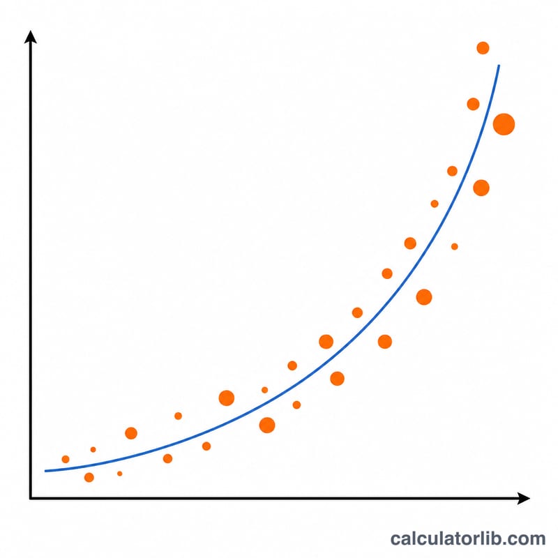
This tool fits an exponential trend curve of the form \(y = A \cdot e^{Bx}\) to a frequency-weighted data set. Each data row is a triple (x, y, f), where f is the frequency or weight — the number of times that observation appears. It returns the fitted coefficients A and B plus the correlation coefficient r of the underlying linear fit. This is pure mathematics and applies identically anywhere, with no region-specific rules.

How to use it

Enter one point per line as x, y, f. The y value must be greater than 0, because the model is linearized by taking its natural logarithm. If you omit the third column, the frequency defaults to 1. Choose how many significant digits to display, then read off A, B, r and the substituted fitted equation.

The formula explained

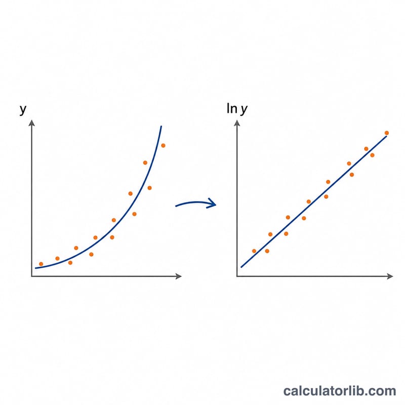
Because ln y = ln A + B·x, fitting the exponential reduces to a weighted linear regression of ln y on x. Using weighted sums where every term is multiplied by the frequency f, define n = Σf, the weighted means x̄ and L̄ (mean of ln y), and the weighted sums of squares Sxx, Syy and cross product Sxy. Then \(B = S_{xy} / S_{xx}\), \(A = e^{\,\bar{L} - B\bar{x}}\), and \(r = S_{xy} / (\sqrt{S_{xx}} \cdot \sqrt{S_{yy}})\). An r near ±1 means a strong fit.

$$y = A \cdot e^{B x}$$ $$\text{where}\quad \left\{ \begin{aligned} B &= \frac{S_{xy}}{S_{xx}} \\ A &= e^{\,\bar{L} - B\bar{x}} \\ S_{xx} &= \textstyle\sum f x^{2} - n\bar{x}^{2} \\ S_{xy} &= \textstyle\sum f x \ln y - n\bar{x}\bar{L} \\ n &= \textstyle\sum f,\quad \bar{x}=\tfrac{\sum f x}{n},\quad \bar{L}=\tfrac{\sum f \ln y}{n} \end{aligned} \right.$$

Advertisement

Taking ln y turns the exponential model into a straight line ln y = ln A + Bx, which the weighted least-squares fit uses.

A frequency-weighted exponential curve y = A·e^(Bx) fitted to data points whose marker size reflects their frequency weight.

Worked example

Take the points (1, 2.7), (2, 7.4), (3, 20.1), (4, 54.6) each with frequency 1, which lie close to \(y = e^{x}\). Here \(\bar{x} = 2.5\), \(\bar{L} \approx 2.49887\), \(S_{xx} = 5\), \(S_{xy} \approx 5.0098\), \(S_{yy} \approx 5.0196\). So \(B \approx 1.0020\), \(A = e^{(2.49887 - 2.5048)} \approx 0.9940\), and \(r \approx 0.9998\). The fitted equation is approximately $$y = 0.9940 \cdot e^{(1.0020 \cdot x)}$$ — essentially \(y = e^{x}\).

FAQ

Why must y be positive? The fit uses ln(y); the logarithm of zero or a negative number is undefined, so such rows are rejected.

What does the frequency f represent? It weights how strongly each point influences the fit — useful for frequency distribution tables where many observations share the same (x, y).

How do I read r? |r| above 0.7 is a strong correlation, 0.4–0.7 moderate, 0.2–0.4 weak, and below 0.2 essentially none.