What this calculator does
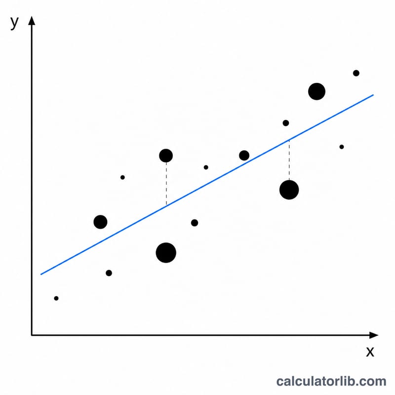
This tool fits a straight line \(y = A + Bx\) to a set of data points using the method of least squares, where each point may carry a frequency or weight f. Frequency weighting lets you summarize repeated observations compactly: instead of listing the same (x, y) pair many times, you give it once with a count. It is a universal, pure-mathematics statistics tool that works the same everywhere.
How to use it
Enter one row per line as x, y, f. The frequency column is optional; if you leave it out, every point is weighted equally (ordinary unweighted regression). Choose how many significant figures you want for the displayed results, then submit. The calculator returns the regression line, the slope B and intercept A, the Pearson correlation coefficient r, the total frequency n, the means of x and y, and the supporting sums Sxx, Syy and Sxy.
The formula explained
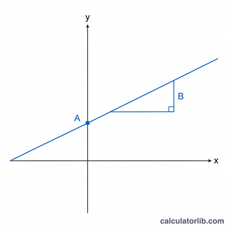
Let the rows be \(i = 1..N\) with values \(x_i\), \(y_i\) and frequency \(f_i\). The total frequency is \(n = \sum f_i\). The weighted means are \(\bar{x} = \sum x_i f_i / n\) and \(\bar{y} = \sum y_i f_i / n\). The sums of squares are $$S_{xx} = \sum x_i^2 f_i - n\cdot\bar{x}^2,$$ $$S_{yy} = \sum y_i^2 f_i - n\cdot\bar{y}^2,$$ and $$S_{xy} = \sum x_i y_i f_i - n\cdot\bar{x}\cdot\bar{y}.$$ The slope is \(B = S_{xy}/S_{xx}\), the intercept is \(A = \bar{y} - B\cdot\bar{x}\), and the correlation is $$r = \frac{S_{xy}}{\sqrt{S_{xx}}\cdot\sqrt{S_{yy}}}.$$
Worked example
For the rows (1,2,1), (2,3,2), (3,5,1), (4,4,2), (5,6,1), (6,7,1): \(n = 8\), \(\bar{x} = 3.375\), \(\bar{y} = 4.25\). Then \(S_{xx} = 19.875\), \(S_{yy} = 19.5\), \(S_{xy} = 18.25\). So $$B = \frac{18.25}{19.875} \approx 0.9182,$$ $$A = 4.25 - 0.9182\cdot 3.375 \approx 1.1509,$$ and \(r \approx 0.9271\) — a strong positive correlation. The fitted line is $$y = 1.1509 + 0.9182\cdot x.$$
FAQ
What does the frequency column do? It weights each point. A point with \(f = 3\) counts as if you observed it three times. Fractional weights are allowed.
What if r cannot be computed? If all x values are equal (\(S_{xx} = 0\)) the slope is undefined, and if either \(S_{xx}\) or \(S_{yy}\) is zero the correlation is undefined because there is no variability.
How is correlation strength judged? Using \(|r|\): above 0.7 is strong, 0.4 to 0.7 moderate, 0.2 to 0.4 weak, and below 0.2 essentially no correlation.


