Frequency-Weighted Curve Regression & Estimation Calculator

Enter Calculation

Data (table input): rows of x, y, f (frequency/weight) 1,2,3 2,4,5 3,5,2 4,8,4 5,9,1 One row per line as x, y, f. Rows with frequency 0 or blank are ignored.

Regression type Linear: y = A + B*x Logarithmic: y = A + B*ln(x) e-Exponential: y = A*e^(B*x) ab-Exponential: y = A*B^x Power: y = A*x^B Inverse: y = A + B/x Quadratic: y = A + B*x + C*x^2

Estimate x (give x, get y) y (give y, get x)

Value to estimate from (=)

Digits (significant) 6 10 14 18 22 26 30 34 38 42 46 50

Formula

Results

Estimated value

7.628571

from frequency-weighted fit (5 active points)

Coefficient A	0.1428571429
Coefficient B	1.8714285714
Coefficient C	0
Correlation coefficient r	0.9878988005

Correlation strength: 0.7 < |r| ≤ 1 strong; 0.4 < |r| < 0.7 moderate; 0.2 < |r| < 0.4 weak; 0 ≤ |r| < 0.2 none. C is non-zero only for the Quadratic model.

What this calculator does

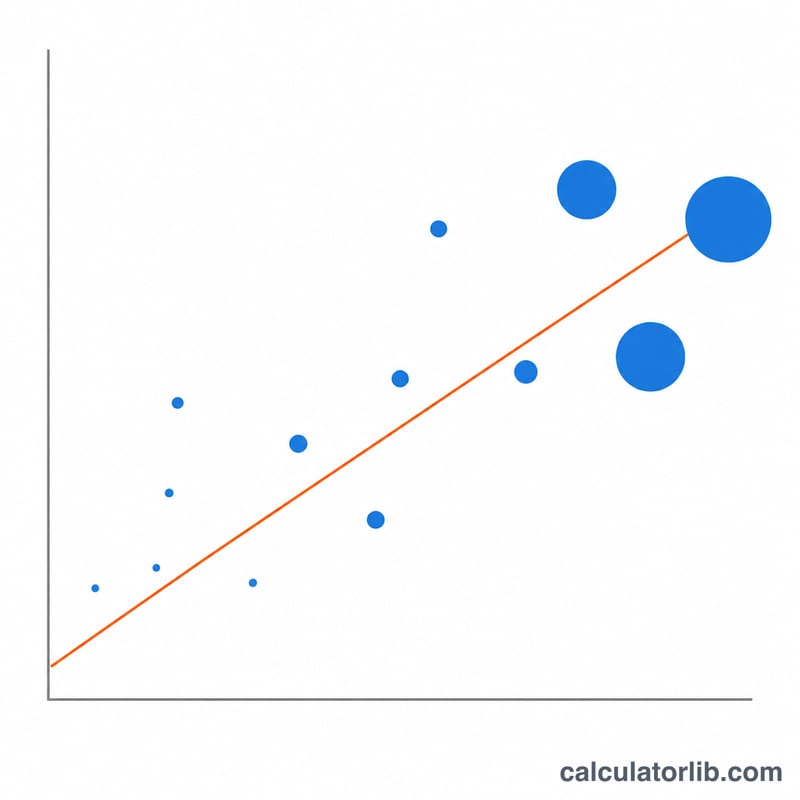
This tool fits a regression curve to a frequency-distribution table of points. Each row is a triple (x, y, f) where x is the independent value, y is the dependent value, and f is the frequency (weight) telling how many times that pair occurred. You pick one of seven curve shapes, the calculator performs a frequency-weighted least-squares fit, then reports the coefficients, the correlation coefficient, and an estimated value. It is pure mathematics and applies anywhere.

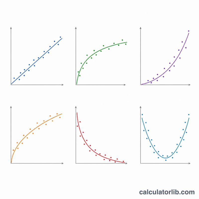
The seven models

Linear: \(y = A + Bx\). Logarithmic: \(y = A + B\ln x\). e-Exponential: \(y = A\,e^{Bx}\). ab-Exponential: \(y = A\,B^{x}\). Power: \(y = A\,x^{B}\). Inverse: \(y = A + \dfrac{B}{x}\). Quadratic: \(y = A + Bx + Cx^{2}\). Every non-quadratic model is linearized to \(Y = a + bX\) with a suitable transform (logarithm or reciprocal) before fitting, then the result is back-transformed into \(A\) and \(B\). The quadratic model is solved directly from the weighted normal equations.

The seven curve models: linear, logarithmic, exponential, power, inverse, and quadratic fits to scattered points.

How to use it

Enter your data, one row per line, as x, y, f. Choose a regression type. Pick whether you want to estimate y from a supplied x, or x from a supplied y, and type the known value. Choose how many significant digits to display. Rows with frequency zero or blank are ignored, and models that need positive x or y (logarithmic, exponential, power) require valid values.

Advertisement

Worked example

Data (x, y, f): (1,2,3), (2,4,5), (3,5,2), (4,8,4), (5,9,1). For the Linear model the weighted sums give \(N=15\), \(S_x=40\), \(S_y=77\), \(S_{xx}=130\), \(S_{xy}=249\). The denominator is $$15 \times 130 - 40^{2} = 350,$$ so $$B = \frac{15 \times 249 - 40 \times 77}{350} = \frac{655}{350} = 1.8714$$ and $$A = \frac{77 - 1.8714 \times 40}{15} = 0.1429.$$ The correlation \(r\) is about 0.9879 (strong). Estimating y at \(x=4\) gives $$0.1429 + 1.8714 \times 4 = 7.6286.$$

Frequency weighting: larger points count more, pulling the fitted line toward heavily weighted data.

FAQ

What does the frequency do? It weights each observation, so a pair with \(f=5\) influences the fit five times as much as a pair with \(f=1\).

Why is C zero? The \(C\) coefficient only exists for the Quadratic model; for the other six it stays zero.

What does r measure for transformed models? It is the Pearson correlation of the linearized \((X, Y)\) variables, so \(|r|=1\) means a perfect fit of the linearized form rather than of the original curve.