
What this calculator does
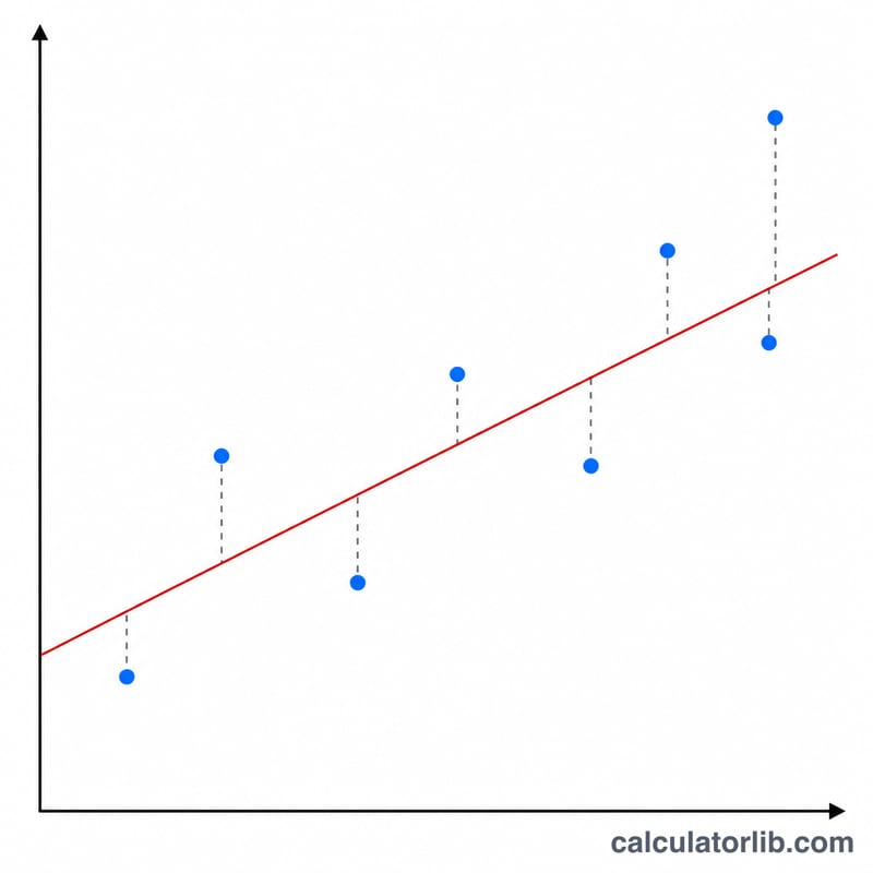
This tool fits a chosen curve-regression model to your table of paired observations (x, y) using the method of least squares. It reports the fitted coefficients (A, B, and C for quadratic), the correlation coefficient r that measures how well the model describes the data, and an estimated value computed directly from the fitted equation. It is a universal mathematics and statistics tool with no region-specific rules.
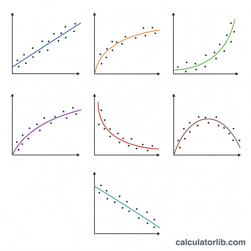
The seven models
You can choose Linear (\(y = A + B\cdot x\)), Logarithmic (\(y = A + B\cdot \ln x\)), e-Exponential (\(y = A\cdot e^{Bx}\)), ab-Exponential (\(y = A\cdot B^{x}\)), Power (\(y = A\cdot x^{B}\)), Inverse (\(y = A + B/x\)), or Quadratic (\(y = A + B\cdot x + C\cdot x^{2}\)). All except the quadratic are fitted by linearizing into the form \(Y = a + b\cdot X\) and applying ordinary least squares; the quadratic is solved from its \(3\times 3\) normal equations.
How to use it
Enter your x values and y values as comma-separated lists of equal length, pick a regression type, choose whether you want to estimate y from x or x from y, and type the known input value. The calculator returns the coefficients, the correlation r, and the estimate.
The formula explained
For the linearized pairs (X, Y): \(b = S_{xy} / S_{xx}\) and \(a = \bar{Y} - b\cdot \bar{X}\), where \(S_{xx} = \sum X^2 - n\bar{X}^2\) and \(S_{xy} = \sum XY - n\bar{X}\bar{Y}\). The correlation is $$r = \frac{S_{xy}}{\sqrt{S_{xx}\cdot S_{yy}}}.$$ Coefficients are then back-substituted (for example \(A = e^a\) in exponential and power models).
Worked example
For x = [1,2,3,4,5,6,7] and y = [3,5,7,8,11,13,14] with a linear fit: \(S_{xx} = 28\), \(S_{xy} = 53\), so $$B = \frac{53}{28} = 1.892857$$ and $$A = 8.714286 - 1.892857\cdot 4 = 1.142857.$$ The correlation is $$r = \frac{53}{\sqrt{28\cdot 101.4286}} = 0.99453.$$ Estimating y at \(x = 64\) gives $$1.142857 + 1.892857\cdot 64 = 122.2857$$ (an extrapolation well beyond the data range).
FAQ
How is r interpreted? Roughly: \(0.7 < |r| \le 1\) strong, \(0.4 < |r| < 0.7\) moderate, \(0.2 < |r| < 0.4\) weak, below \(0.2\) negligible.
Why are some models rejected? Logarithmic and power models require \(x > 0\), exponential and power models require \(y > 0\), and inverse requires \(x \ne 0\), because of the log or reciprocal transforms.
Can I extrapolate? Yes, but estimates outside the observed data range are extrapolations and should be treated with caution.


