Curve Regression Analysis Calculator

Enter Calculation

Data (x,y pairs) 1,2 2,3 3,5 4,4 5,6 Enter one (x, y) pair per line, e.g. 1,2. Lines may be separated by new lines or semicolons.

Regression type Linear: y = A + B*x Logarithmic: y = A + B*ln(x) e-Exponential: y = A*e^(B*x) ab-Exponential: y = A*B^x Power: y = A*x^B Inverse: y = A + B/x Quadratic: y = A + B*x + C*x^2

Display digits

Results

Fitted equation

y = 1.3 + 0.9x

based on 5 data points

A (intercept / scale)	1.3
B (slope / exponent)	0.9
Correlation coefficient r	0.9
Mean of x (working space)	3
Mean of y (working space)	4

Correlation strength guide (|r|):

• 0.7 < |r| ≤ 1 — strong correlation
• 0.4 < |r| < 0.7 — moderate correlation
• 0.2 < |r| < 0.4 — weak correlation
• 0 ≤ |r| < 0.2 — no correlation

What this calculator does

The Curve Regression Analysis Calculator fits a chosen mathematical curve to a table of (x, y) data points. It returns the fitted coefficients (A, B and, for the quadratic model, C), the explicit fitted equation, and the correlation coefficient r that measures how well the curve matches your data. This is pure statistics and applies identically anywhere — all values are dimensionless numbers with no units.

Supported models

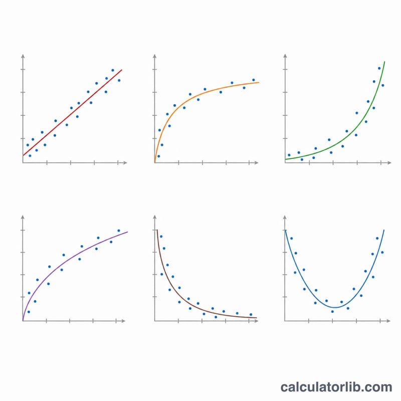
You can fit seven curve families: Linear (\(y = A + B\cdot x\)), Logarithmic (\(y = A + B\cdot \ln x\)), e-Exponential (\(y = A\cdot e^{B\cdot x}\)), ab-Exponential (\(y = A\cdot B^{x}\)), Power (\(y = A\cdot x^{B}\)), Inverse (\(y = A + B/x\)) and Quadratic (\(y = A + B\cdot x + C\cdot x^{2}\)). Every non-quadratic model is fitted by transforming the variables (taking logs or reciprocals), running ordinary least squares, and back-transforming the coefficients.

The six supported regression models and their characteristic curve shapes.

How to use it

Type your data with one (x, y) pair per line, for example 1,2. Pick a regression type from the dropdown, set the number of display digits, and submit. Logarithmic and power models require all \(x > 0\); the exponential and power models require all \(y > 0\); the inverse model requires \(x \neq 0\). The quadratic model needs at least three points.

Advertisement

The formula explained

For transformed variables u and v, least squares gives slope $$B = \frac{N\cdot\sum uv - \sum u\cdot\sum v}{N\cdot\sum u^{2} - (\sum u)^{2}}$$ and intercept $$A = \frac{\sum v - B\cdot\sum u}{N}.$$ The correlation r uses the same numerator over the square root of the product of the x and y variation terms. For non-linear models, A and B are recovered with \(\exp(\ldots)\) after fitting in log space.

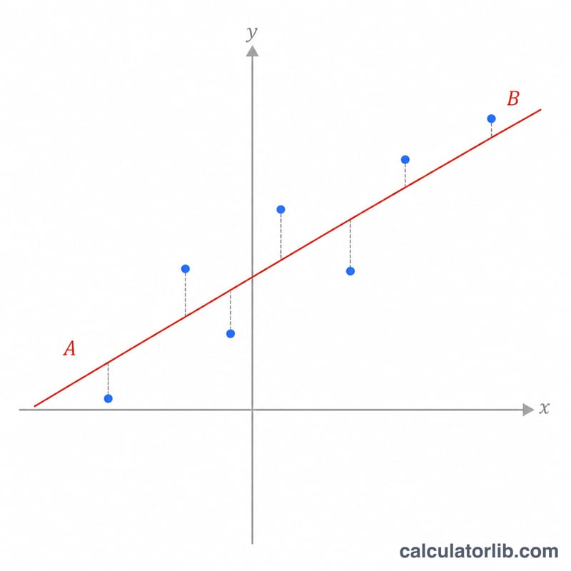
Worked example (Linear)

Data: (1,2), (2,3), (3,5), (4,4), (5,6). Here \(N=5\), \(\sum x=15\), \(\sum y=20\), \(\sum x^{2}=55\), \(\sum xy=69\), \(\sum y^{2}=90\). Then $$B = \frac{5\cdot 69 - 15\cdot 20}{5\cdot 55 - 225} = \frac{45}{50} = 0.9$$ and $$A = \frac{20 - 0.9\cdot 15}{5} = 1.3.$$ The fitted line is \(y = 1.3 + 0.9x\) with $$r = \frac{45}{\sqrt{50\cdot 50}} = 0.9,$$ a strong positive correlation.

Advertisement

Least-squares fitting minimizes the vertical distances between points and the line.

FAQ

What does r mean? Values of \(|r|\) above 0.7 indicate strong correlation, 0.4–0.7 moderate, 0.2–0.4 weak, and below 0.2 essentially none.

Why does the exponential model reject negative y? Fitting happens on \(\ln(y)\), which is undefined for non-positive values, so those models require \(y > 0\).

Which model should I pick? Plot your data first: roughly straight lines suit linear, accelerating growth suits exponential or power, and curves with a single bend suit quadratic.