What is the Weighted Curve Regression Calculator?
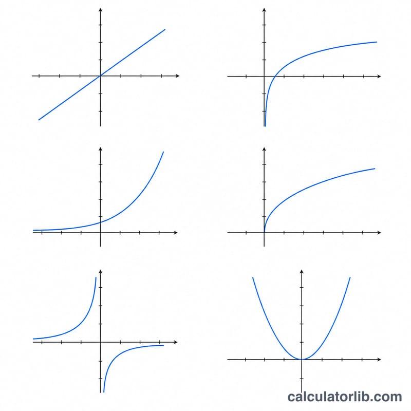
This universal statistics tool fits a chosen curve model to a frequency-weighted data set. You supply rows of (x, y, frequency) and pick a model — Linear, Logarithmic, e-Exponential, ab-Exponential, Power, Inverse, or Quadratic — and it returns the fitted coefficients (A, B, and C for quadratic), the correlation coefficient r, and a plain-language interpretation of the correlation strength. It is pure mathematics, so it applies anywhere with no jurisdiction or units.
How to use it
Enter your data three numbers per row separated by commas or spaces: x, y, frequency. The frequency (weight) is how many times that (x,y) pair occurs; if you leave it blank it defaults to 1 (unweighted). Choose a model and submit. Use at least 2 distinct points (3 for quadratic). Logarithmic and Power models require \(x > 0\); the exponential and power models require \(y > 0\); the inverse model requires \(x \ne 0\).
The formula explained
Most models are fit by linearization: transform x and/or y into (X, Y) so the relationship becomes a straight line \(Y = a + b\cdot X\), then run a weighted least-squares fit with weights \(w_i = f_i\). With \(N = \Sigma w\), the slope is $$b = \frac{N\cdot S_{xy} - S_x\cdot S_y}{N\cdot S_{xx} - S_x^2}$$ and intercept $$a = \frac{S_y - b\cdot S_x}{N},$$ where the sums are weighted. The Pearson r is computed in the transformed space. For e-Exponential and ab-Exponential we fit \(\ln(y)\) against x; for Power we fit \(\ln(y)\) against \(\ln(x)\); Inverse fits y against \(1/x\). Quadratic solves the 3×3 weighted normal equations directly and reports the multiple correlation \(R = \sqrt{1 - SSE/SST}\).
Worked example
Points (x,y,f): (1,2,1),(2,3,1),(3,5,1),(4,4,1),(5,6,1), Linear model. \(N=5\), \(S_x=15\), \(S_y=20\), \(S_{xx}=55\), \(S_{xy}=69\), \(S_{yy}=90\). Then $$b = \frac{5\cdot 69 - 15\cdot 20}{5\cdot 55 - 225} = \frac{45}{50} = 0.9$$ and $$a = \frac{20 - 0.9\cdot 15}{5} = 1.3.$$ So \(y = 1.3 + 0.9x\), with $$r = \frac{45}{\sqrt{50\cdot 50}} = 0.9$$ — a strong correlation.
FAQ
What does the frequency column do? It weights each point: a frequency of 3 counts that pair three times in every sum, exactly like a frequency distribution table. A frequency of 0 drops the row.
How is correlation strength classified? By \(|r|\): above 0.7 is strong, 0.4–0.7 moderate, 0.2–0.4 weak, and 0.2 or below is no correlation.
Why might I get an error? If all X values are identical the denominator is zero and no unique line exists, or if your data violates a model's domain (e.g. a non-positive y with an exponential model).


