What this calculator does
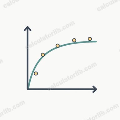
This tool fits a logarithmic regression curve of the form \(y = A + B\cdot\ln(x)\) to a table of observations, where every row carries a frequency (weight) f. Frequency weighting lets you enter grouped or repeated data compactly: instead of listing the same (x, y) pair many times, you write it once with its count f. The method is pure statistics and works identically anywhere — no units or country rules apply.
How to use it
Enter one observation group per line as x y f. The frequency column is optional; if you leave it off, each row counts once (f = 1). Every x must be greater than zero because the natural logarithm of x is taken. Provide at least two rows with distinct x values so the line is determined. Pick a display precision (default 10 significant digits) — this only changes rounding of the shown numbers, never the underlying computation.
The formula explained
With groups i = 1..m, let \(n = \sum f_i\). The weighted means are \(\text{meanLnX} = \frac{\sum f_i\cdot\ln x_i}{n}\) and \(\text{meanY} = \frac{\sum f_i\cdot y_i}{n}\). The weighted sums of squares are $$S_{xx} = \sum f_i(\ln x_i)^2 - n\cdot\text{meanLnX}^2,$$ $$S_{yy} = \sum f_i y_i^2 - n\cdot\text{meanY}^2,$$ $$S_{xy} = \sum f_i\cdot\ln x_i\cdot y_i - n\cdot\text{meanLnX}\cdot\text{meanY}.$$ Then \(B = S_{xy}/S_{xx}\), \(A = \text{meanY} - B\cdot\text{meanLnX}\), and $$r = \frac{S_{xy}}{\sqrt{S_{xx}}\cdot\sqrt{S_{yy}}}.$$
Worked example
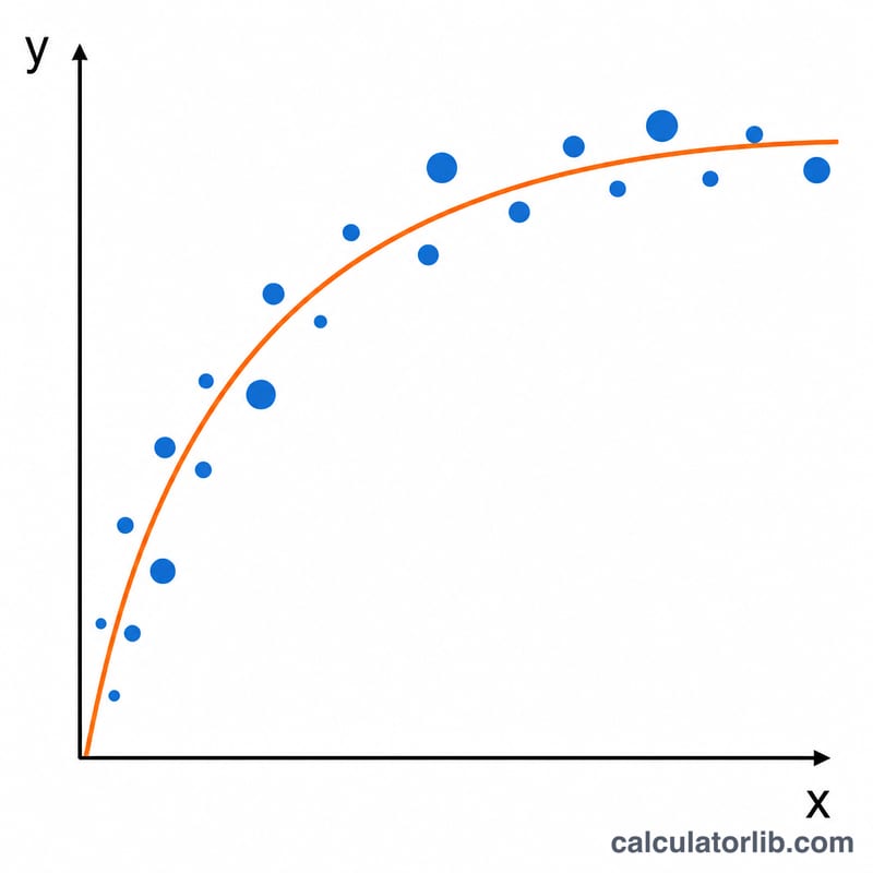
Using five rows with all f = 1 — (1,2), (2,3), (3,3), (4,4), (5,4) — we get \(\text{meanLnX} = 0.9574984\), \(\text{meanY} = 3.2\), \(S_{xx} = 1.6154888\), \(S_{yy} = 2.8\), \(S_{xy} = 2.0382328\). So \(B = 1.2616933\), \(A = 1.9919295\), and \(r = 0.9583567\). The fitted curve is $$y = 1.9919 + 1.2617\cdot\ln(x)$$ with a strong correlation.
FAQ
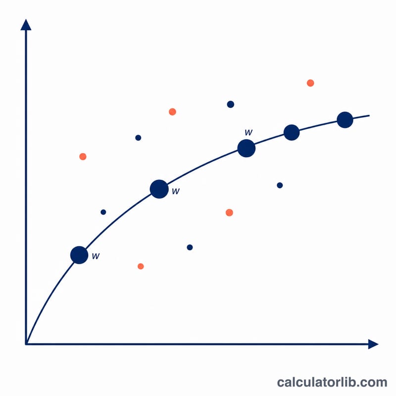
What does the frequency column do? It weights each row. A row with f = 5 is treated as five identical observations, so it influences the fit five times as much as a row with f = 1.
How do I read r? \(|r|\) above 0.7 is strong, 0.4–0.7 moderate, 0.2–0.4 weak, and below 0.2 essentially no correlation.
Why does it say "cannot fit"? A fit requires at least two distinct x values (otherwise \(S_{xx} = 0\)) and a positive total frequency. All x values must be greater than zero so \(\ln(x)\) is defined.


