
What this calculator does
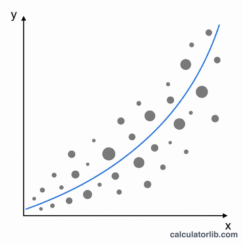
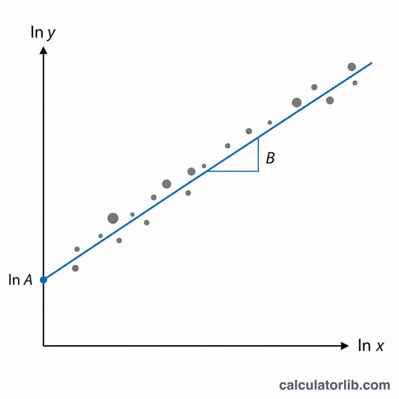
This tool fits a power-law trend line of the form \(y = A\cdot x^{B}\) to a set of data points, where each point (x, y) can carry a frequency or weight f. It is a frequency-weighted least-squares regression performed in natural-log space, which turns the power curve into a straight line \(\ln y = \ln A + B\cdot\ln x\). The method is pure mathematics and statistics, so it applies everywhere with no regional rules.
How to use it
Enter the x values, y values and frequencies as three comma-separated lists of equal length. Every x and y must be strictly positive (the logarithm is undefined for zero or negative numbers) and every frequency should be zero or greater. Pick the number of significant digits for the displayed output, then read off the fitted coefficient A, the exponent B and the Pearson correlation coefficient r.
The formula explained
For each row let \(X = \ln x\) and \(Y = \ln y\). With total weight \(n = \sum f\), the weighted means are \(\overline{\ln x} = \frac{\sum f\cdot\ln x}{n}\) and \(\overline{\ln y} = \frac{\sum f\cdot\ln y}{n}\). The weighted sums of squares are $$S_{xx} = \sum f(\ln x)^2 - n\cdot\overline{\ln x}^{\,2},$$ $$S_{yy} = \sum f(\ln y)^2 - n\cdot\overline{\ln y}^{\,2},$$ $$S_{xy} = \sum f(\ln x)(\ln y) - n\cdot\overline{\ln x}\cdot\overline{\ln y}.$$ Then $$B = \frac{S_{xy}}{S_{xx}}, \quad A = \exp\!\left(\overline{\ln y} - B\cdot\overline{\ln x}\right) \quad\text{and}\quad r = \frac{S_{xy}}{\sqrt{S_{xx}}\cdot\sqrt{S_{yy}}}.$$ Each point effectively counts as if repeated f times.
Worked example
Take x = [1, 2, 3, 4, 5] and y = [1, 4, 9, 16, 25] (exactly \(y = x^2\)) with all frequencies 1. The computation gives \(S_{xx} \approx 1.615494\), \(S_{xy} \approx 3.230987\) and \(S_{yy} \approx 6.461972\), so $$B = \frac{3.230987}{1.615494} = 2, \quad A = \exp(0) = 1 \quad\text{and}\quad r = 1.$$ The result \(y = 1\cdot x^2\) is a perfect fit, as expected.
FAQ
What does the correlation coefficient mean? \(|r|\) near 1 means a strong power-law relationship; 0.4–0.7 is moderate, 0.2–0.4 is weak and below 0.2 is essentially none.
Why must x and y be positive? The fit uses natural logarithms, which are only defined for positive numbers, so non-positive points are skipped.
What if all x values are equal? Then \(S_{xx} = 0\) and the exponent B cannot be determined, so the calculator reports an error.


