What is logarithmic regression?
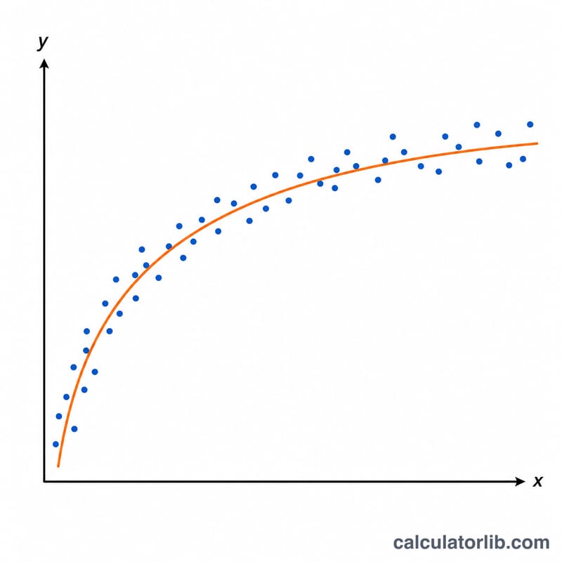
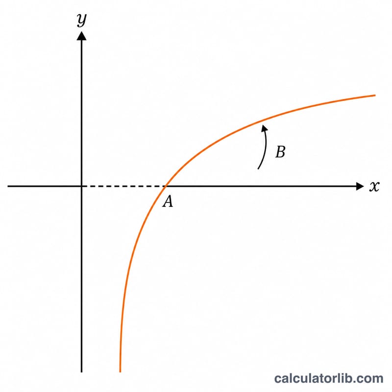
Logarithmic regression fits a curve of the form \(y = A + B\cdot\ln(x)\) to your data. It is useful when a quantity grows quickly at first and then levels off, so that equal multiplicative steps in x produce roughly equal additive steps in y. By taking the natural logarithm of every x value, the problem becomes an ordinary straight-line (least-squares) fit in the transformed variable \(u = \ln(x)\).
How to use this calculator
Enter your data in the table area, one (x, y) pair per line, separated by a comma or space. Every x value must be strictly positive because \(\ln(x)\) is undefined for zero or negative numbers; such rows and blank lines are ignored. Choose how many significant digits to display, then read off the fitted intercept A, coefficient B, the correlation coefficient r, and the means.
The formula explained
Let \(u_i = \ln(x_i)\). Compute the means of u and y, then the sums of squares \(S_{xx} = \sum (u-\bar{u})^2\), \(S_{yy} = \sum (y-\bar{y})^2\), and the cross-product \(S_{xy} = \sum (u-\bar{u})(y-\bar{y})\). The slope is $$B = \frac{S_{xy}}{S_{xx}},$$ the intercept is $$A = \bar{y} - B\cdot\bar{u},$$ and the correlation is $$r = \frac{S_{xy}}{\sqrt{S_{xx}}\cdot\sqrt{S_{yy}}}.$$ Note that the displayed "mean x" is the geometric mean \(\exp(\bar{u})\), not the arithmetic mean, because the fit is performed in log space.
Worked example
For the points (1, 2.0), (2, 4.0), (3, 5.0), (4, 5.5), (5, 6.0): \(\text{meanLnX} = 0.957498\), \(\text{meanY} = 4.5\), \(S_{xx} = 1.615493\), \(S_{yy} = 10.0\), \(S_{xy} = 4.003192\). So \(B = 2.4780\), \(A = 2.1273\), and \(r = 0.9963\) (strong correlation). The fitted line is $$y = 2.1273 + 2.4780\cdot\ln(x),$$ and the geometric mean $$x = \exp(0.957498) = 2.6051.$$
FAQ
Why is the "mean x" not the average of my x values? Because the regression is computed on \(\ln(x)\), the natural center of the x data in this model is the geometric mean \(\exp(\text{mean of }\ln x)\), which is what is reported.
How do I read the correlation coefficient r? \(|r|\) above 0.7 indicates a strong relationship, 0.4-0.7 moderate, 0.2-0.4 weak, and below 0.2 essentially no correlation.
What if all my x values are equal? Then \(S_{xx} = 0\) and the slope is undefined (division by zero), so the fit cannot be computed; you need at least two distinct x values.


