Inverse Regression Calculator (y = A + B/x)

Enter Calculation

Data (table input): one point per line as x, y 1, 6.0 2, 3.0 3, 2.0 4, 1.5 5, 1.2 Enter each (x, y) pair on its own line, comma or space separated. x must be non-zero. Minimum 2 points.

Significant digits 6 10 14 18 22 26 30 34 38 42 46 50

Results

Fitted inverse regression equation

y = 0.0 + (6.0)/x

model: y = A + B/x

A (intercept)	0.0
B (numerator coefficient)	6.0
Correlation coefficient r	1.0
Data points used (n)	5

Correlation strength: strong correlation (|r| = 1).
Fitted curve points (x, y): 1.0,6.0; 1.1,5.455; 1.2,5.0; 1.3,4.615; 1.4,4.286; 1.5,4.0; 1.6,3.75; 1.7,3.529; 1.8,3.333; 1.9,3.158; 2.0,3.0; 2.1,2.857; 2.2,2.727; 2.3,2.609; 2.4,2.5; 2.5,2.4; 2.6,2.308; 2.7,2.222; 2.8,2.143; 2.9,2.069; 3.0,2.0; 3.1,1.935; 3.2,1.875; 3.3,1.818; 3.4,1.765; 3.5,1.714; 3.6,1.667; 3.7,1.622; 3.8,1.579; 3.9,1.538; 4.0,1.5; 4.1,1.463; 4.2,1.429; 4.3,1.395; 4.4,1.364; 4.5,1.333; 4.6,1.304; 4.7,1.277; 4.8,1.25; 4.9,1.224; 5.0,1.2

What is inverse regression?

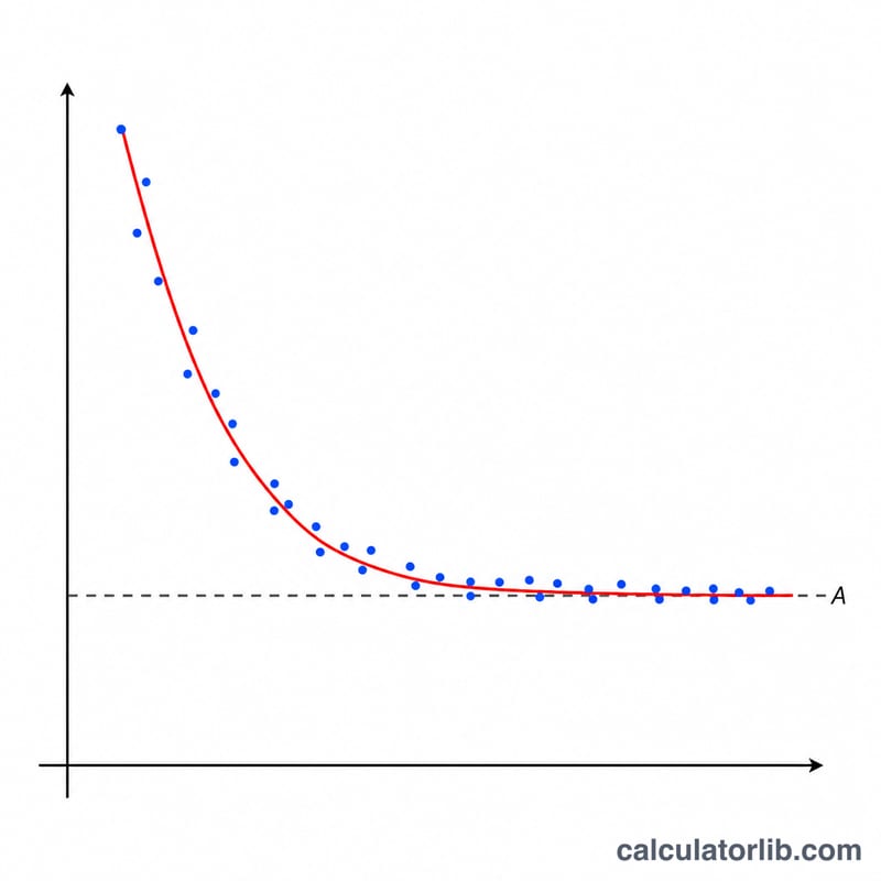
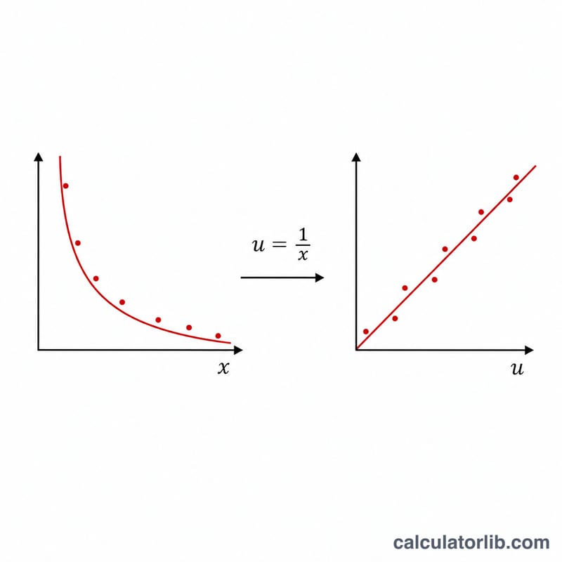
Inverse regression (also called reciprocal regression) fits a set of paired observations to the model \(y = A + \frac{B}{x}\). This curve is the natural choice when a quantity falls off in proportion to \(\frac{1}{x}\) — for example, when the response is high for small \(x\) and tends toward a constant baseline \(A\) as \(x\) grows large. Because the model is linear in the transformed predictor \(u = \frac{1}{x}\), it can be solved exactly with ordinary least squares. This is a universal mathematics and statistics tool: the formulas are the same everywhere.

The inverse model \(y = A + \frac{B}{x}\) bends sharply for small \(x\) and levels off toward \(A\) for large \(x\).

How to use it

Enter your data with one point per line in the form x, y (comma or space separated). You need at least two points, and every \(x\) must be non-zero because the model uses \(\frac{1}{x}\). Pick the number of significant digits for the displayed output (this affects formatting only, not the internal computation). The calculator returns the intercept \(A\), the numerator coefficient \(B\), the correlation coefficient \(r\) between \(\frac{1}{x}\) and \(y\), the fully substituted equation, and a sampled fitted curve you can plot against your scatter points.

The formula explained

For each point compute \(u_i = \frac{1}{x_i}\), then run a simple linear regression of \(y\) on \(u\). Using the means \(\bar{u}\) and \(\bar{y}\), form $$S_{uu} = \sum u^2 - n\cdot\bar{u}^2,$$ $$S_{uy} = \sum (u\cdot y) - n\cdot\bar{u}\cdot\bar{y},$$ and $$S_{yy} = \sum y^2 - n\cdot\bar{y}^2.$$ Then the slope is \(B = \frac{S_{uy}}{S_{uu}}\), the intercept is \(A = \bar{y} - B\cdot\bar{u}\), and the correlation is $$r = \frac{S_{uy}}{\sqrt{S_{uu}} \cdot \sqrt{S_{yy}}}.$$

Advertisement

Substituting \(u = \frac{1}{x}\) turns the inverse model into a straight line, fit by ordinary least squares.

Worked example

For \(x = [1, 2, 3, 4, 5]\) and \(y = [6, 3, 2, 1.5, 1.2]\): \(\bar{u} = 0.456667\), \(\bar{y} = 2.74\), \(S_{uu} = 0.420889\), \(S_{uy} = 2.525333\), \(S_{yy} = 15.152\). So $$B = \frac{2.525333}{0.420889} = 6.000,$$ $$A = 2.74 - 6\cdot 0.456667 = 0.000,$$ and $$r = \frac{2.525333}{0.648759 \cdot 3.892557} = 1.000.$$ The fit is exactly \(y = \frac{6}{x}\), a perfect inverse relationship.

FAQ

Why must \(x\) be non-zero? The model uses \(\frac{1}{x}\), which is undefined at \(x = 0\), so any such row is skipped and reported.

What does \(r\) mean here? It measures how well \(\frac{1}{x}\) predicts \(y\) linearly: \(|r|\) above 0.7 is strong, 0.4–0.7 moderate, 0.2–0.4 weak, below 0.2 no correlation.

When does the fit fail? If all \(x\) values are equal, every \(\frac{1}{x}\) is identical, \(S_{uu} = 0\), and the slope cannot be determined.