What is the von Mises distribution?
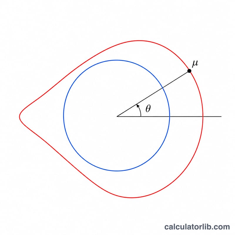
The von Mises distribution is the circular analogue of the normal (Gaussian) distribution. It models angles or directions on a circle, characterized by a mean direction \(\mu\) and a concentration parameter \(\kappa\). When \(\kappa\) is large the distribution is tightly peaked around \(\mu\); when \(\kappa = 0\) it becomes the uniform distribution on the circle. This calculator is a universal mathematical tool — it applies everywhere and uses radians throughout.
How to use this calculator
Choose what you want: the probability density f, the lower cumulative probability P (the CDF), or the upper cumulative probability \(Q = 1 - P\). Enter the mean direction \(\mu\) (radians), the concentration \(\kappa \ge 0\), and the angle \(x\) (radians) at which to evaluate. Press calculate to see all three quantities, with your selected one highlighted.
The formula explained
The probability density function is $$f(\text{x}) = \frac{e^{\kappa\cos\left(\text{x} - \mu\right)}}{2\pi\, I_{0}\!\left(\kappa\right)}$$ where \(I_0(\kappa)\) is the modified Bessel function of the first kind of order 0, computed from the convergent series $$I_0(\kappa) = \sum \frac{(\kappa/2)^{2m}}{(m!)^2}$$ The cumulative probability \(P(x)\) is the integral of f from \(\mu-\pi\) up to \(x\); here it is obtained by Simpson's rule over 2000 subintervals after wrapping \(z = x - \mu\) into \([-\pi, \pi]\), so P ranges from 0 at \(z = -\pi\) to 1 at \(z = +\pi\). Q is simply \(1 - P\).
$$F(\text{x}) = \int_{-\pi}^{\,\text{x} - \mu} \frac{e^{\kappa\cos\theta}}{2\pi\, I_{0}\!\left(\kappa\right)}\, d\theta$$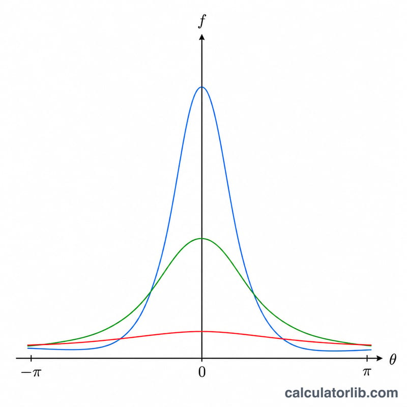
Worked example
Take \(\mu = 0\), \(\kappa = 1\), \(x = 0\). Then \(I_0(1) \approx 1.2660658778\) and \(\cos(0) = 1\), so \(e^{1} = 2.71828\). The density is $$f = \frac{2.71828}{2\pi \cdot 1.26607} \approx 0.3417 \text{ per radian}$$ By symmetry of f about \(\mu = 0\), exactly half the mass lies below \(x = 0\), giving \(P(0) = 0.5\) and \(Q(0) = 0.5\).
FAQ
What unit is the density in? The PDF has units of 1/radian, since it integrates to 1 over a \(2\pi\)-radian circle.
What happens when \(\kappa = 0\)? The distribution becomes uniform on the circle: \(f(x) = 1/(2\pi) \approx 0.159155\) for every \(x\), and \(P(x)\) increases linearly.
Can I enter x outside \([\mu-\pi, \mu+\pi]\)? Yes. The density is \(2\pi\)-periodic in \(x\), and the CDF wraps \(z = x - \mu\) into \([-\pi, \pi]\) before integrating.


