What is the Weibull distribution?
The Weibull distribution is one of the most flexible continuous probability distributions and a cornerstone of reliability engineering, life-data analysis and survival modeling. By tuning two parameters — a shape parameter m (also written k or beta) and a scale parameter eta (also written lambda or a, the characteristic life) — it can model failure rates that decrease, stay constant or increase over time. This calculator uses the standard 2-parameter scale form with location fixed at zero, so its support is \(x \ge 0\).
How to use this calculator
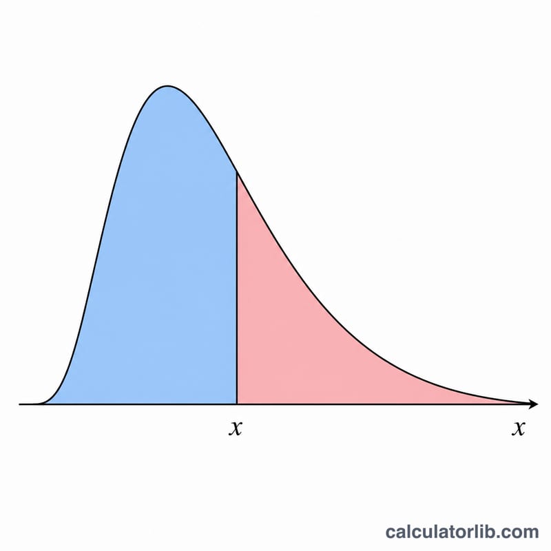
Enter the value x at which you want to evaluate the distribution (\(x \ge 0\)), the shape parameter m (\(> 0\)) and the scale parameter eta (\(> 0\)). The tool returns three results: the probability density \(f(x)\), the lower cumulative probability \(P(X \le x)\) (the CDF), and the upper cumulative probability \(P(X > x)\) (the survival or reliability function). Note that \(F(x) + R(x)\) always equals 1.
The formulas explained
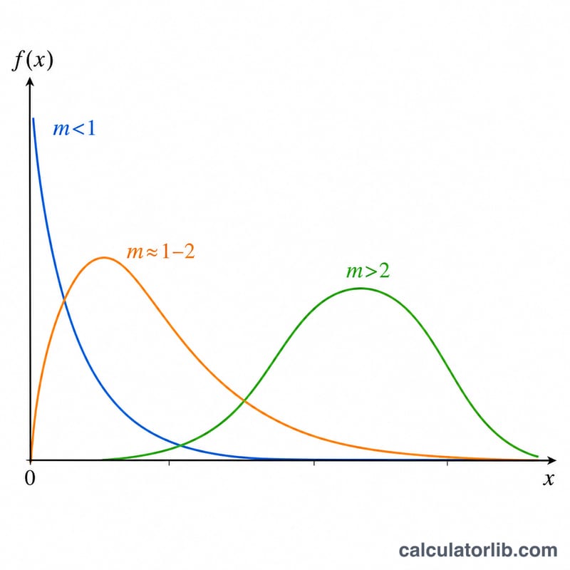
Let \(z = x / \eta\). The density is $$f(x) = \frac{m}{\eta} \cdot z^{m-1} \cdot e^{-z^{m}}$$ The cumulative distribution function is $$F(x) = 1 - e^{-z^{m}}$$ and the survival function is $$R(x) = e^{-z^{m}}$$ The shape parameter controls the hazard behaviour: \(m = 1\) reduces to the exponential distribution (constant failure rate, mean \(\eta\)), \(m = 2\) gives the Rayleigh distribution, and \(m\) near 3.6 approximates a bell-shaped normal curve.
Worked example
Take \(x = 1.5\), \(m = 2\), \(\eta = 1\). Then \(z = 1.5\) and \(z^m = 2.25\), so \(e^{-2.25} = 0.105399\). The upper cumulative probability \(R = 0.105399\) and the lower cumulative $$F = 1 - 0.105399 = 0.894601$$ The density is $$f = \frac{2}{1} \cdot 1.5^{1} \cdot 0.105399 = 0.316198$$
FAQ
Why is \(F(\eta)\) about 0.632 for every shape? When \(x = \eta\), \(z = 1\) so \(z^m = 1\) and \(F = 1 - e^{-1} = 0.6321\), independent of \(m\). That is why \(\eta\) is called the characteristic life.
What happens for \(x < 0\)? The 2-parameter Weibull has support \([0, \infty)\), so \(f(x) = 0\), \(F(x) = 0\) and \(R(x) = 1\) there.
Does scale need units? Inputs are pure numbers; \(x\) and \(\eta\) should share the same units (e.g. hours), but the calculation itself is dimensionless.


