
What this calculator does
This tool returns the percentile, also called the quantile, of a continuous uniform distribution defined on an interval from a lower bound a to an upper bound b. Given a cumulative probability you provide, it finds the value x on the interval at which that probability is reached. Because the uniform distribution spreads probability evenly across [a, b], the answer is a simple, exact linear interpolation.
How to use it
Pick a cumulative mode. Choose Lower cumulative P if your probability means P(X ≤ x) (the area to the left). Choose Upper cumulative Q if it means P(X ≥ x) (the area to the right). Enter the probability as a number between 0 and 1, then enter the lower bound a and the upper bound b, with a ≤ b. The calculator returns the percentile x and the effective lower-tail probability p it used internally.
The formula explained
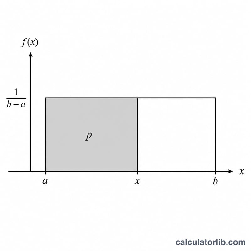
For a continuous uniform variable on [a, b], the cumulative distribution function is \(F(x) = (x - a) / (b - a)\). Inverting it gives the quantile:
$$x = a + p \cdot (b - a)$$where \(p\) is the lower-tail probability. In lower mode \(p\) equals your P directly. In upper mode, since \(Q = 1 - F(x)\), the lower-tail equivalent is \(p = 1 - Q\). The result always lies between a and b: \(p = 0\) gives \(x = a\) and \(p = 1\) gives \(x = b\). If a equals b the distribution is degenerate and \(x = a\) for any valid probability.
Worked example
Lower mode, P = 0.2, a = 1, b = 4. Then \(p = 0.2\) and
$$x = 1 + 0.2 \cdot (4 - 1) = 1 + 0.6 = 1.6$$Switching to upper mode with Q = 0.2 gives \(p = 0.8\) and
$$x = 1 + 0.8 \cdot 3 = 3.4$$checking, \(P(X \ge 3.4) = (4 - 3.4)/3 = 0.2\), as required.
FAQ
What is the difference between P and Q? P is the area to the left of x (probability of being at or below x); Q is the area to the right (probability of being at or above x). They sum to 1.
What if my probability is outside 0 to 1? Probabilities must lie in [0, 1]; values outside this range are clamped to the nearest boundary before computing.
Does this work for the discrete uniform distribution? No. This calculator models the continuous uniform distribution; for the discrete case quantiles step between integer values.


