What this calculator does
This tool computes the percentile (also called the quantile or percent point) of a Cauchy distribution, also known as the Lorentz distribution. Given a cumulative probability and the distribution's two parameters — the location x0 (the median and peak position) and the scale γ (gamma, the half-width at half-maximum) — it returns the value x at which that probability is reached. This is pure mathematics and applies identically everywhere.
How to use it
First choose the cumulative mode. Select Lower if your probability P is a left-tail probability, \(P = \text{Prob}(X \le x)\). Select Upper if your probability Q is a right-tail probability, \(Q = \text{Prob}(X \ge x)\). Then enter the probability as a fraction strictly between 0 and 1 (for example 0.95 for the 95th percentile), the location parameter x0, and the scale parameter γ (which must be positive). The calculator returns the corresponding x.
The formula explained
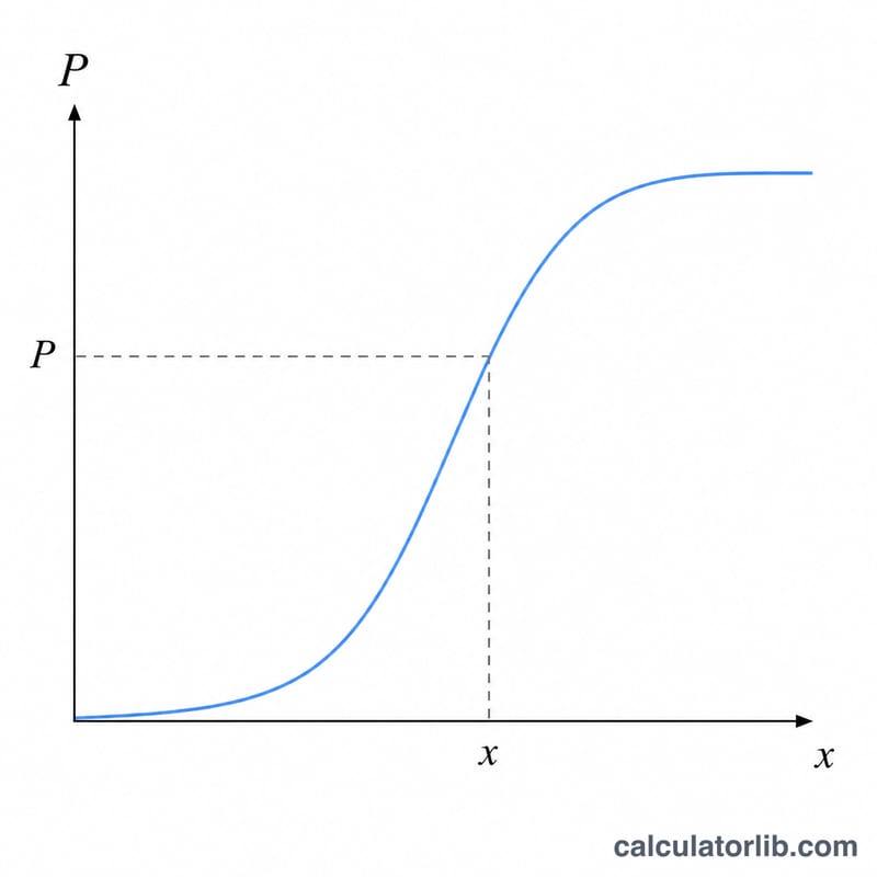
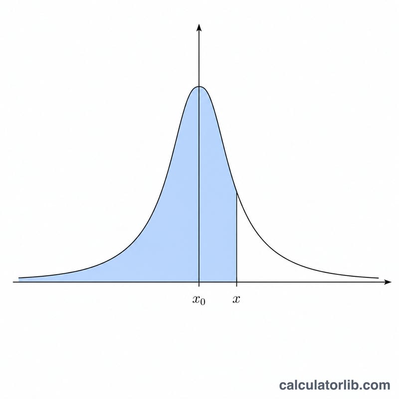
The cumulative distribution function of the Cauchy distribution is \(F(x) = \tfrac{1}{2} + \tfrac{1}{\pi}\cdot\arctan\!\left(\tfrac{x - x_0}{\gamma}\right)\). Inverting it gives the quantile function $$x = x_0 + \gamma \cdot \tan\!\left(\pi\left(P - \tfrac{1}{2}\right)\right),$$ where P is the lower cumulative probability. If you entered an upper probability Q, the tool first converts it with \(P = 1 - Q\). At \(P = 0.5\) the result is exactly x0; as P approaches 0 or 1 the result diverges toward minus or plus infinity, reflecting the famously heavy tails of the Cauchy distribution (it has no finite mean or variance).
Worked example
For the lower 95th percentile with \(x_0 = 0\) and \(\gamma = 1\): \(P = 0.95\), so $$x = 0 + 1\cdot\tan(\pi\cdot 0.45) = \tan(1.41372\ \text{rad}) \approx 6.31375.$$ Checking: \(F(6.31375) = 0.5 + \tfrac{1}{\pi}\cdot\arctan(6.31375) = 0.5 + 0.45 = 0.95\). With \(x_0 = 2\), \(\gamma = 3\) and \(P = 0.75\): $$x = 2 + 3\cdot\tan(\pi\cdot 0.25) = 2 + 3\cdot 1 = 5.0.$$
FAQ
What is the difference between lower and upper mode? They are complementary: an upper probability of 0.05 gives the same x as a lower probability of 0.95.
Why must the probability be strictly between 0 and 1? At exactly 0 or 1 the quantile is plus or minus infinity, which has no finite numeric value.
Can the scale be negative? No. The scale γ must be greater than 0; it represents a half-width and a negative value is undefined.


