What is the F-distribution percent point?
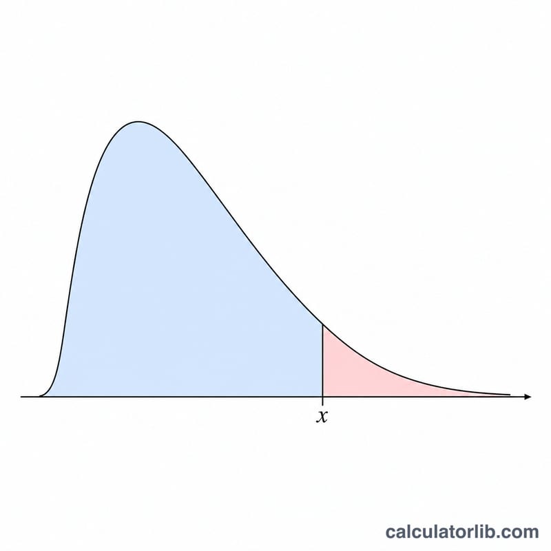
The F-distribution percent point (also called the inverse F, the quantile, or the critical value) is the value x such that the cumulative F-distribution with degrees of freedom d1 (numerator) and d2 (denominator) equals a chosen probability. It is the inverse of the F-distribution CDF and is exactly the critical value you look up in F-tables for ANOVA, regression overall significance tests, and variance-ratio (equality-of-variances) tests.
How to use the calculator
Pick a cumulative mode. Choose Lower cumulative P if your probability is \(P = \Pr(F \le x)\) — for example P = 0.95 returns the value below which 95% of the distribution lies. Choose Upper cumulative Q if you have a tail probability \(Q = \Pr(F > x)\) — for example Q = 0.05 returns the usual upper 5% critical value. Enter the probability (strictly between 0 and 1), the numerator degrees of freedom d1, and the denominator degrees of freedom d2, then submit.
The formula explained
The F-distribution CDF is written using the regularized incomplete beta function I: with \(a = d_1/2\), \(b = d_2/2\) and the substitution \(w = d_1 \cdot x / (d_1 \cdot x + d_2)\), we have $$\text{F-CDF}(x) = I_w(a, b).$$ To invert it, the calculator solves \(I_w(a, b) = \text{targetP}\) for \(w\) by bisection on \((0, 1)\), evaluating \(I_w\) with a Lanczos log-gamma and the Numerical Recipes continued fraction. It then back-substitutes $$x = \frac{d_2 \cdot w}{d_1 \cdot (1 - w)}.$$ In Upper mode the target probability becomes \(\text{targetP} = 1 - Q\).
Worked example
For P = 0.95, d1 = 5, d2 = 10 we seek the upper 5% F critical value. With \(a = 2.5\) and \(b = 5\), inverting \(I_w(2.5, 5) = 0.95\) gives \(w \approx 0.6245\), and $$x = \frac{10 \times 0.6245}{5 \times 0.3755} \approx 3.3258,$$ matching the tabulated \(F_{0.05}(5, 10) = 3.3258\).
FAQ
What is the difference between P and Q? P is the lower-tail (cumulative) probability up to x; Q is the upper-tail probability beyond x. They are related by \(P = 1 - Q\).
Why must the probability be strictly between 0 and 1? A probability of 0 corresponds to the quantile \(x = 0\) and a probability of 1 corresponds to \(x \to \infty\), neither of which is a finite, meaningful critical value.
Can degrees of freedom be non-integer? Yes — the math works for any positive real d1 and d2, though ANOVA applications normally use integers.


