What this calculator does
This is a pure-mathematics statistics tool for the exponential distribution. It computes the percent point (also called the quantile or inverse cumulative distribution function) x given a cumulative probability and the scale parameter b. The exponential distribution is universal — it models waiting times between independent events that occur at a constant average rate — so this calculator applies identically everywhere.
How to use it
Choose the cumulative mode. Select Lower cumulative P if your entered probability is the lower-tail probability P (the area to the left of x), or Upper cumulative Q if it is the upper-tail probability Q (the area to the right). Enter the probability value between 0 and 1, then enter the scale parameter b, which must be positive. The scale b equals the distribution mean, where \(b = 1/\lambda\). The result x is reported in the same units as b.
The formula explained
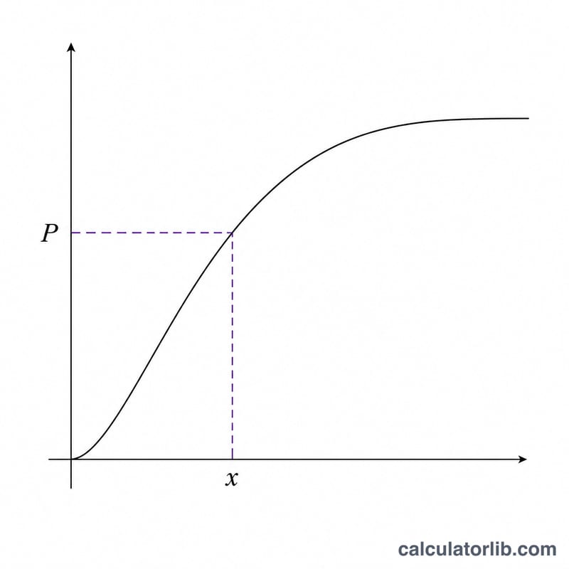
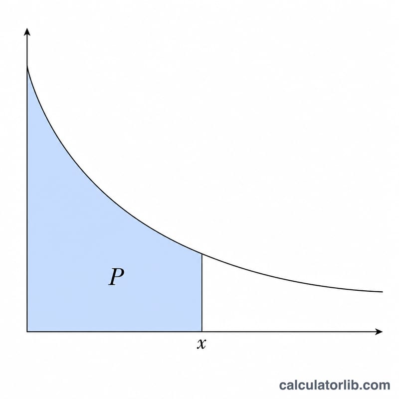
The exponential probability density is \(f(x) = (1/b)\cdot\exp(-x/b)\) for \(x \ge 0\). Its lower cumulative function is \(P(x) = 1 - \exp(-x/b)\), and its upper cumulative function is \(Q(x) = \exp(-x/b)\). Inverting these gives the percent point. In lower mode, $$x = -b\cdot\ln(1 - P).$$ In upper mode, $$x = -b\cdot\ln(Q).$$ Both reduce to \(x = -b\cdot\ln(Q)\) where Q is the upper-tail probability, with ln being the natural logarithm (base e).
Worked example
Suppose cumulativeMode is Lower, probability P = 0.4 and scale b = 1. Then $$x = -1\cdot\ln(1 - 0.4) = -\ln(0.6) = 0.51083.$$ Check: \(P(0.51083) = 1 - \exp(-0.51083) = 1 - 0.6 = 0.4\). Correct.
FAQ
What is the scale parameter b? It is the mean of the distribution, \(b = 1/\lambda\), where \(\lambda\) is the rate. A larger b means events take longer on average.
Why can the result be infinite? In lower mode P = 1 (or upper mode Q = 0) corresponds to the entire tail, which pushes x to infinity. The calculator reports this case rather than returning a number.
Lower vs upper mode — which should I pick? Use lower mode when you know the cumulative probability up to x (a percentile such as the median). Use upper mode when you know a survival or exceedance probability beyond x.


