What this calculator does
The inverse chi-square percent point calculator finds the quantile x of the chi-square distribution given a cumulative probability and the degrees of freedom. In other words, it solves the inverse cumulative distribution function (inverse CDF), returning the critical value used in hypothesis tests, confidence intervals and goodness-of-fit analysis. This is universal pure mathematics and applies identically everywhere.
How to use it
Pick a cumulative mode. Choose Lower tail if your probability P is P(X ≤ x) (the area to the left). Choose Upper tail if your probability Q is P(X > x) (the area to the right, the common form for critical values). Enter the probability between 0 and 1, then the degrees of freedom (nu), which must be positive. The calculator returns x.
The formula
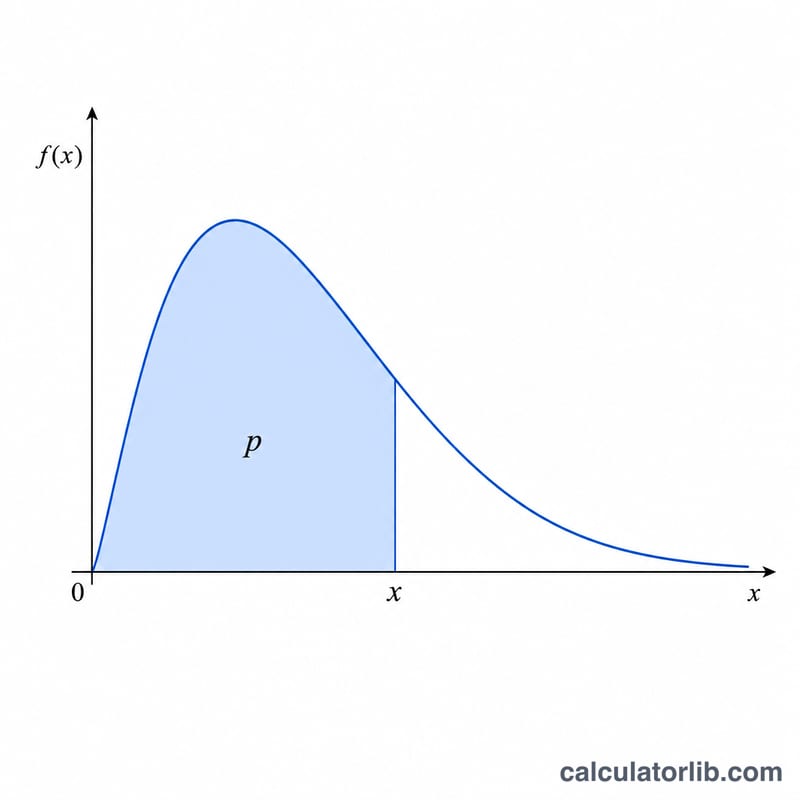
The chi-square CDF with nu degrees of freedom is \(F(x;\ \nu) = P\!\left(\tfrac{\nu}{2},\tfrac{x}{2}\right)\), where \(P\) is the regularized lower incomplete gamma function. For the lower tail we solve $$x = F^{-1}\!\left(\text{P};\ \nu\right) \quad\text{such that}\quad P\!\left(\tfrac{\nu}{2},\tfrac{x}{2}\right) = \text{P}$$ For the upper tail we set \(p_{\text{eff}} = 1 - Q\) and solve $$x = F^{-1}\!\left(1 - \text{Q};\ \nu\right) \quad\text{such that}\quad P\!\left(\tfrac{\nu}{2},\tfrac{x}{2}\right) = 1 - \text{Q}$$ The equation is inverted numerically with a robust bracketing bisection on \(g(x) = F(x) - p_{\text{eff}}\).
Worked example
Upper tail, \(Q = 0.05\), \(\nu = 10\). Then \(p_{\text{eff}} = 1 - 0.05 = 0.95\), so we solve \(F(x;\ 10) = 0.95\), i.e. \(\text{regularizedGammaP}(5,\ x/2) = 0.95\). The root is \(x \approx 18.307\), the familiar chi-square critical value for 10 degrees of freedom at the 5% upper-tail level.
FAQ
What does degrees of freedom mean here? It is the shape parameter \(\nu\) of the chi-square distribution; the equivalent gamma shape is \(\nu/2\) with scale 2.
Lower vs upper tail? Lower tail uses the area left of x; upper tail uses the area right of x. Critical-value tables usually quote upper-tail probabilities.
Why might x be 0 or very large? As the effective lower-tail probability approaches 0, x approaches 0; as it approaches 1, x grows without bound.


