What is the Chi-Square Distribution Percentile Calculator?
This tool finds the percentage point (also called the quantile or percentile, often written as a critical value) of the chi-square distribution. Given a cumulative probability and the degrees of freedom, it returns the value x at which the chi-square cumulative distribution function (CDF) equals your target probability. It is the inverse of the chi-square CDF and is widely used in hypothesis testing, goodness-of-fit tests, contingency-table analysis, and confidence intervals for variance.
How to use it
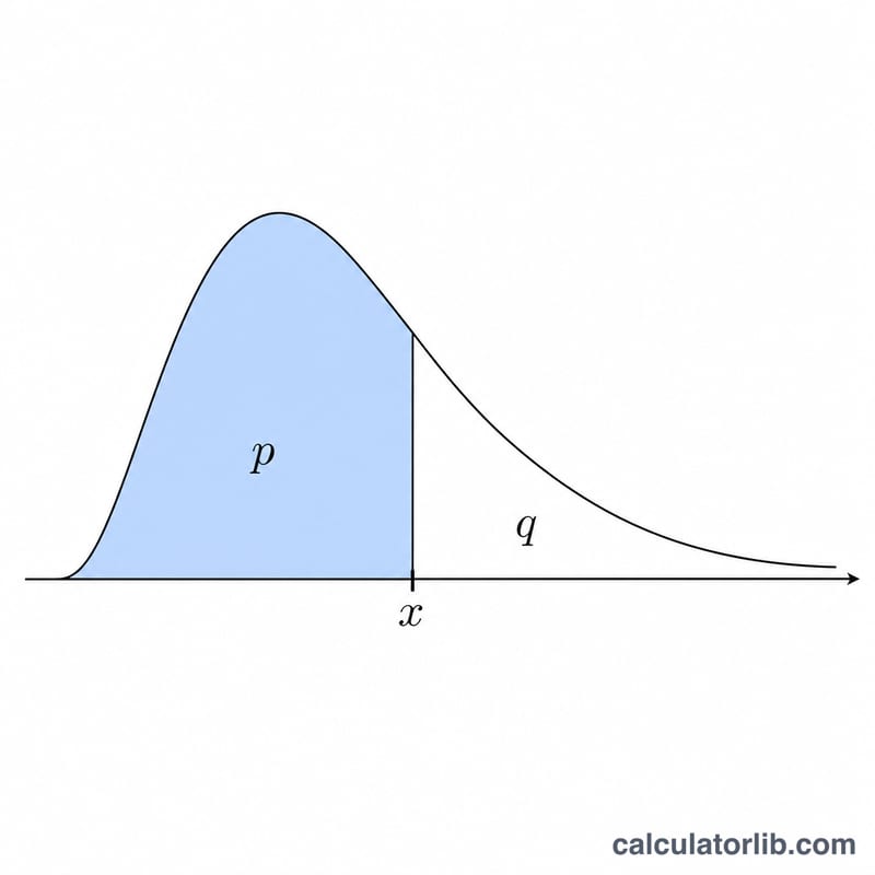
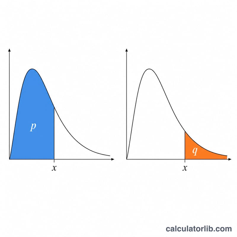
Pick a cumulative mode. Choose "Lower cumulative P" when your probability is \(P = P(X \le x)\) (the area to the left of x). Choose "Upper cumulative Q" when your probability is the tail area \(Q = P(X > x)\) — the typical significance level alpha in a one-sided test. Enter the probability (strictly between 0 and 1) and the degrees of freedom (nu, also written k). The calculator returns the chi-square value x.
The formula explained
The chi-square CDF with nu degrees of freedom is the regularized lower incomplete gamma function: \(F(x; \nu) = \text{regularizedGammaP}\left(\frac{\nu}{2}, \frac{x}{2}\right)\). We need the inverse. Setting \(a = \frac{\nu}{2}\) and the target probability p (where p = P in lower mode, or p = 1 - Q in upper mode), we solve $$x_p = F^{-1}\!\left(\text{p}\,;\,\nu\right)\ \text{such that}\ P\!\left(\frac{\nu}{2},\,\frac{x_p}{2}\right) = \text{p}$$ \(\text{regularizedGammaP}(a, z) = p\) for z, then \(x = 2z\). The solver combines a series expansion and a continued fraction for the incomplete gamma, with a Newton/bisection root finder for guaranteed convergence.
Worked example
Take lower mode, \(P = 0.95\), \(\nu = 10\). Then \(a = 5\) and we solve \(\text{regularizedGammaP}(5, z) = 0.95\), giving \(z \approx 9.1535\), so $$x = 2z \approx 18.307$$ This matches the classic critical value \(\chi^2(0.95, 10) = 18.307\). Using upper mode with \(Q = 0.05\) and \(\nu = 10\) gives \(p = 1 - 0.05 = 0.95\) and the same \(x \approx 18.307\).
FAQ
What is the difference between P and Q? P is the area to the left of x (lower tail); Q is the area to the right (upper tail), and \(P + Q = 1\).
Can degrees of freedom be non-integer? Yes. The gamma-based formula works for any \(\nu > 0\), though most statistical tables use integers.
What probability range is valid? Strictly \(0 < \text{probability} < 1\). At 0 the quantile is 0; as the probability approaches 1 the quantile grows without bound.


