
What is the Beta Distribution Calculator?
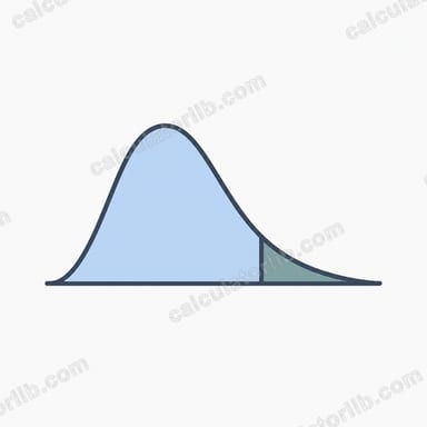
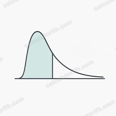
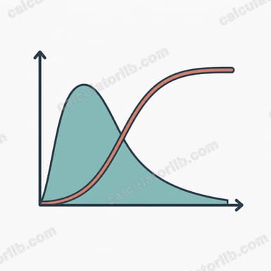
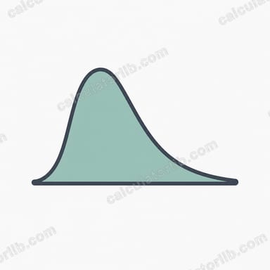
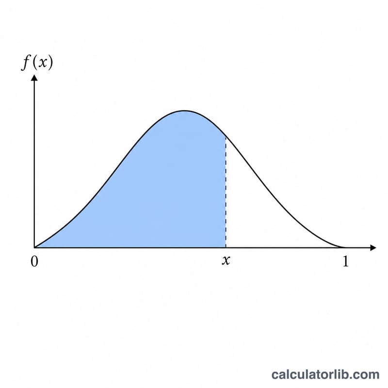
The Beta distribution is a continuous probability distribution defined on the interval [0, 1], governed by two positive shape parameters, a and b. It is widely used in Bayesian statistics (as a conjugate prior for probabilities), reliability analysis, project scheduling (PERT), and modelling proportions. This calculator evaluates the probability density function \(f(x)\), the lower cumulative probability \(P(x)\) (the cumulative distribution function), and the upper cumulative probability \(Q(x)\) (the survival function) across a grid of x values, and draws a line plot of the chosen function.
How to use it
Choose which function to compute, enter the shape parameters a and b (both must be greater than 0), then set the starting x, the step size, and the number of rows. The tool evaluates the selected function at \(x = \text{initialX}\), \(\text{initialX} + \text{step}\), \(\text{initialX} + 2\cdot\text{step}\), and so on. With the defaults (start 0, step 0.01, 101 rows) you get a full sweep from \(x = 0.00\) to \(x = 1.00\). The result shows the value at the first x, a complete table, and a graph.
The formula explained
The density is $$f(x,a,b) = \frac{x^{\,a-1}\,(1-x)^{\,b-1}}{B(a,b)},$$ where the beta function $$B(a,b)=\frac{\Gamma(a)\,\Gamma(b)}{\Gamma(a+b)}$$ normalises the area to 1. For numerical stability we work with the log-gamma function (Lanczos approximation) so \(B(a,b)\) is computed as \(\exp\!\big(\ln\Gamma(a) + \ln\Gamma(b) - \ln\Gamma(a+b)\big)\). The lower cumulative probability equals the regularized incomplete beta function \(I_x(a,b)\), computed with the Numerical Recipes continued-fraction method (betacf/betai). The upper cumulative probability is simply \(Q = 1 - P\).
Worked example
Take \(a = 2\), \(b = 3\), \(x = 0.3\). Here $$B(2,3) = \frac{1\cdot 2}{24} = 0.0833333,$$ so $$f(0.3) = 12 \cdot 0.3 \cdot 0.7^2 = 12 \cdot 0.147 = 1.764.$$ The lower cumulative probability \(P(0.3) = I_{0.3}(2,3) = 0.3483\), and the upper cumulative probability \(Q(0.3) = 1 - 0.3483 = 0.6517\).
Key Formulas & Moments
The Beta distribution is a continuous probability distribution defined on the support interval \([0,1]\), governed by two positive shape parameters \(a>0\) and \(b>0\). Its probability density function is
$$f(x)=\frac{x^{a-1}\,(1-x)^{b-1}}{B(a,b)},\qquad 0\le x\le 1.$$The normalizing constant \(B(a,b)\) is the beta function, which is expressed through gamma functions as
$$B(a,b)=\int_0^1 t^{a-1}(1-t)^{b-1}\,dt=\frac{\Gamma(a)\,\Gamma(b)}{\Gamma(a+b)}.$$The principal moments and shape descriptors are summarized below.
| Quantity | Formula | Conditions |
|---|---|---|
| Mean | \(\mu=\dfrac{a}{a+b}\) | all \(a,b>0\) |
| Variance | \(\sigma^2=\dfrac{ab}{(a+b)^2\,(a+b+1)}\) | all \(a,b>0\) |
| Mode | \(\dfrac{a-1}{a+b-2}\) | \(a>1,\ b>1\) |
| Skewness | \(\gamma_1=\dfrac{2\,(b-a)\,\sqrt{a+b+1}}{(a+b+2)\,\sqrt{ab}}\) | all \(a,b>0\) |
For example, with \(a=2\) and \(b=5\) the mean is \(\mu=\dfrac{2}{2+5}=\dfrac{2}{7}\approx 0.2857\) and the variance is \(\sigma^2=\dfrac{2\cdot 5}{(7)^2(8)}=\dfrac{10}{392}\approx 0.0255\). Since both parameters exceed 1, the mode is \(\dfrac{2-1}{2+5-2}=\dfrac{1}{5}=0.2\). When \(a=b\) the distribution is symmetric about \(x=0.5\) and the skewness is zero; when \(b>a\) it is right-skewed and when \(a>b\) it is left-skewed. The special case \(a=b=1\) reduces to the standard uniform distribution on \([0,1]\).
Definitions & Glossary
- Shape parameter a
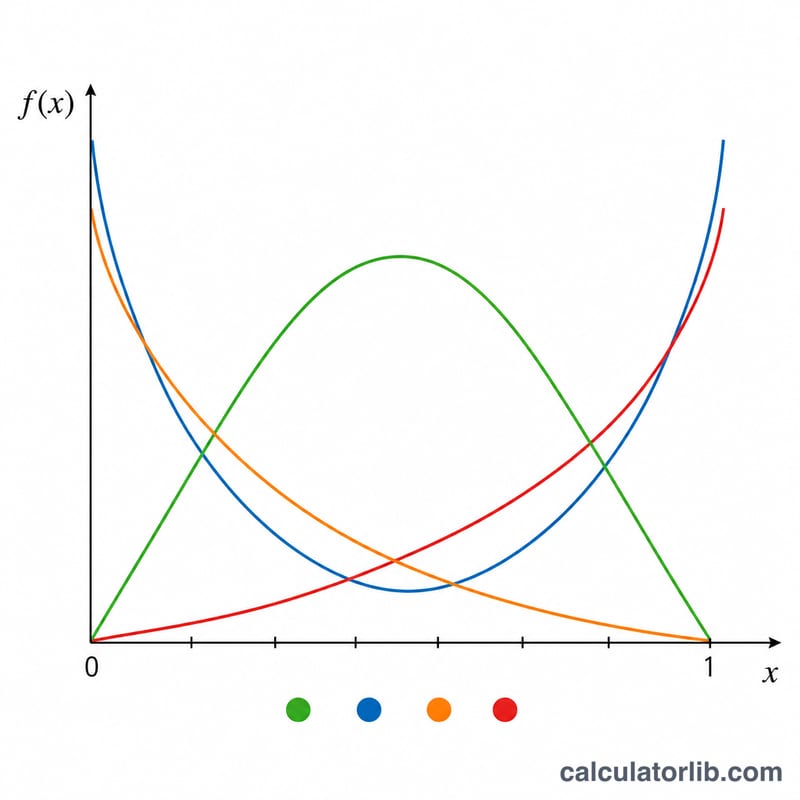
- The first positive shape parameter (\(a>0\)). It controls the behaviour of the density near \(x=0\): values \(a<1\) push mass toward 0 (density diverges), \(a=1\) gives a finite endpoint, and \(a>1\) makes the density vanish at 0. Larger \(a\) relative to \(b\) shifts the mean toward 1.
- Shape parameter b
- The second positive shape parameter (\(b>0\)). It governs the density near \(x=1\) in the mirror-image way that \(a\) governs the behaviour near 0. Larger \(b\) relative to \(a\) shifts the mean toward 0.
- Probability density function f(x)
- The relative likelihood of the random variable taking the value \(x\), given by \(f(x)=\dfrac{x^{a-1}(1-x)^{b-1}}{B(a,b)}\) for \(0\le x\le 1\) and 0 elsewhere. The area under \(f(x)\) over \([0,1]\) equals 1.
- Lower cumulative probability P(x) / CDF
- The cumulative distribution function, \(P(x)=\Pr(X\le x)=\displaystyle\int_0^x f(t)\,dt\). It equals the regularized incomplete beta function \(I_x(a,b)\) and increases monotonically from 0 at \(x=0\) to 1 at \(x=1\).
- Upper cumulative probability Q(x) / survival function
- The complementary (tail) probability, \(Q(x)=\Pr(X> x)=1-P(x)\). It decreases from 1 at \(x=0\) to 0 at \(x=1\).
- Beta function B(a,b)
- The normalizing constant of the distribution, \(B(a,b)=\int_0^1 t^{a-1}(1-t)^{b-1}\,dt=\dfrac{\Gamma(a)\Gamma(b)}{\Gamma(a+b)}\). It is symmetric: \(B(a,b)=B(b,a)\).
- Gamma function \(\Gamma(z)\)
- The continuous extension of the factorial, defined by \(\Gamma(z)=\int_0^\infty t^{z-1}e^{-t}\,dt\), with \(\Gamma(n)=(n-1)!\) for positive integers \(n\) and the recurrence \(\Gamma(z+1)=z\,\Gamma(z)\).
- Regularized incomplete beta function \(I_x(a,b)\)
- The ratio \(I_x(a,b)=\dfrac{1}{B(a,b)}\displaystyle\int_0^x t^{a-1}(1-t)^{b-1}\,dt\), which ranges from 0 to 1 and is exactly the CDF of the Beta distribution, so \(P(x)=I_x(a,b)\).
FAQ
What range can x take? The Beta distribution lives on [0, 1]; outside that interval the density is 0.
What do a and b control? They shape the curve: \(a = b = 1\) gives the uniform distribution, large values concentrate mass near the mean \(\frac{a}{a+b}\), and values below 1 push mass toward the edges.
Why might the density be very large near the edges? When \(a < 1\) the density diverges as x approaches 0, and when \(b < 1\) it diverges as x approaches 1; these endpoints are handled with limit rules.