What is the Lévy distribution?
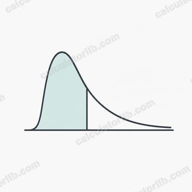
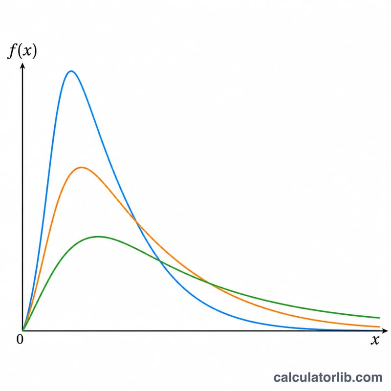
The Lévy distribution is a continuous, heavy-tailed probability distribution defined for values greater than a location parameter mu. It has two parameters: the location parameter mu, which shifts where the support begins, and the scale parameter c (which must be positive), which stretches the distribution. It is a stable distribution and appears in physics (Brownian motion first-passage times), finance, and the study of anomalous diffusion. Notably, both its mean and variance are infinite, which is why this tool reports density and cumulative probabilities rather than summary moments.
How to use this calculator
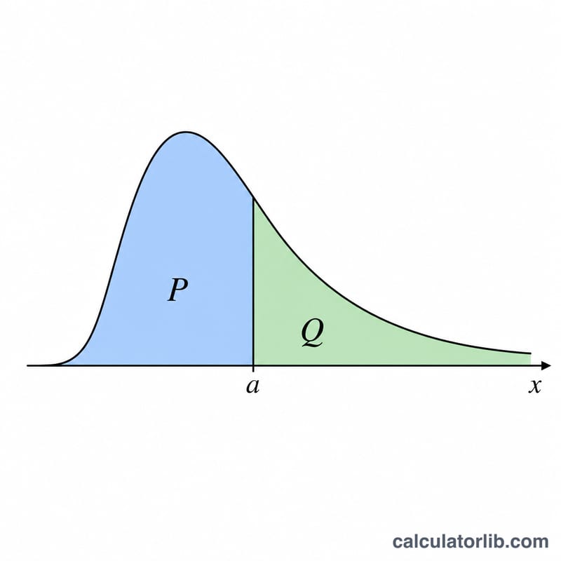
Choose which curve to display: the probability density function f, the lower cumulative probability P, or the upper cumulative probability Q. Enter the location parameter mu and a positive scale parameter c. Then define the range of x to evaluate using a starting value, an increment (step), and a number of points. The calculator evaluates x at each point, prints f, P and Q at the first x, and plots the selected function as a curve across the range.
The formula explained
Let \(s = x - mu\). For \(s > 0\) the density is $$f(x) = \sqrt{\frac{c}{2\pi}} \cdot e^{-\frac{c}{2s}} \cdot s^{-3/2}.$$ The lower cumulative distribution is $$P(x) = \operatorname{erfc}\!\left(\sqrt{\frac{c}{2s}}\right),$$ where erfc is the complementary error function, and the upper (survival) function is $$Q(x) = 1 - P(x) = \operatorname{erf}\!\left(\sqrt{\frac{c}{2s}}\right).$$ For x at or below mu there is no probability mass, so \(f = 0\), \(P = 0\) and \(Q = 1\). The error function is evaluated with the Abramowitz & Stegun 7.1.26 rational approximation.
Worked example
With \(mu = 0\), \(c = 1\) and \(x = 1\): \(s = 1\), so $$f = \sqrt{\frac{1}{2\pi}} \cdot e^{-0.5} = 0.398942 \cdot 0.606531 \approx 0.24197.$$ The argument \(z = \sqrt{1/2} = 0.70711\), \(\operatorname{erf}(z) \approx 0.68269\), so \(P = \operatorname{erfc}(z) \approx 0.31731\) and \(Q \approx 0.68269\) — the standard Lévy(0,1) values.
FAQ
Why must c be greater than 0? The scale parameter sets the spread of the distribution; a non-positive c makes the density undefined, so the calculator requires \(c > 0\).
What happens for x below mu? The distribution has no support there, so \(f = 0\), the lower cumulative probability \(P = 0\), and the upper cumulative probability \(Q = 1\).
Why are there no mean and variance? The Lévy distribution is so heavy-tailed that its mean and variance diverge to infinity, so no finite summary moments are reported.


