

What is the Laplace distribution?
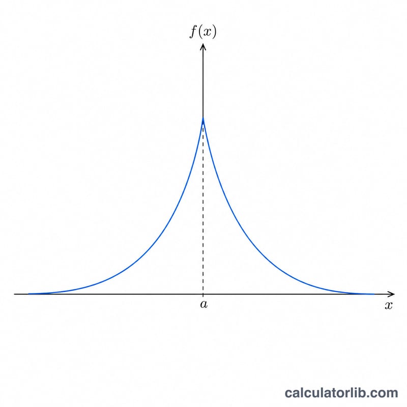
The Laplace distribution, also called the double-exponential distribution, is a continuous probability distribution that looks like two exponential curves placed back to back at a central peak. It is governed by two numbers: a location parameter a (the mean, median and mode all coincide there) and a scale parameter b (which must be greater than zero and controls how quickly the tails decay). It appears in signal processing, robust statistics, Bayesian LASSO priors and models where data have heavier tails than the normal distribution.
How to use this calculator
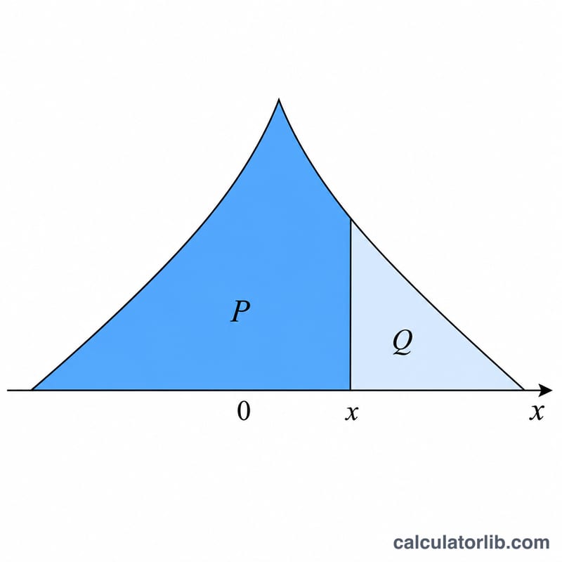
Pick which quantity you want with the Function selection radio: the probability density f, the lower cumulative probability P (the CDF), or the upper cumulative probability Q. Enter the location parameter a and a positive scale parameter b. Then define the x sequence with three fields: x initial value, x increment and repeat count. The points are generated as \(x_k = x_{\text{Initial}} + k\cdot x_{\text{Step}}\) for k = 0 to count−1. The tool evaluates the chosen function at every point, draws a line graph and lists each (x, value) pair in a table. The hero value shown is the function at the first x.
The formula explained
The density is $$f(x,a,b) = \frac{1}{2\,\text{b}}\, e^{-\frac{\left| x - \text{a} \right|}{\text{b}}}$$ The absolute value makes the curve symmetric about a. Integrating gives the CDF: for x < a, \(P = 0.5\cdot e^{(x-a)/b}\); for x ≥ a, \(P = 1 - 0.5\cdot e^{-(x-a)/b}\). The upper tail is simply \(Q = 1 - P\). At the peak x = a you get \(f = \frac{1}{2b}\) and \(P = Q = 0.5\).
Worked example
With a = 0, b = 0.7 evaluated at x = 1: $$f = \frac{1}{1.4}\cdot e^{-1/0.7} = 0.714286 \times 0.239651 \approx 0.17118$$ Since x ≥ a, \(P = 1 - 0.5\cdot e^{-1.42857} = 0.88017\) and \(Q = 0.11983\). Notice \(P + Q = 1\) exactly, a handy self-check.
FAQ
Why must b be positive? The density divides by 2b and the exponent uses b; if b ≤ 0 the function is undefined, so the calculator rejects it.
What does Q represent? \(Q(x)\) is the probability that a random value exceeds x, i.e. the right-tail or survival probability, equal to \(1 - P(x)\).
How many points can I plot? Any positive integer up to 1000. The defaults (start −5, step 0.1, 101 points) span x from −5 to +5.