What is the Student's t-Distribution Calculator?
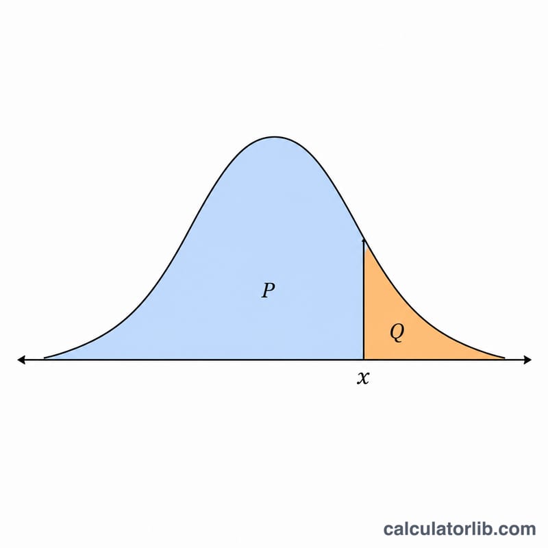
This tool evaluates the Student's t-distribution for a given value x (the t statistic) and degrees of freedom ν. It returns three quantities: the probability density f(x), the lower cumulative probability P(T ≤ x), and the upper cumulative probability Q = P(T > x) = 1 − P. This is pure mathematics and applies universally; no region-specific rules are involved.
How to use it
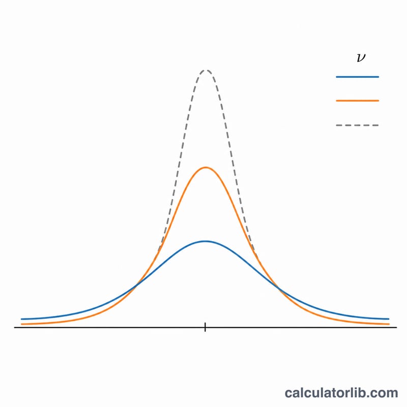
Enter any real number for x (it may be negative) and a positive number for the degrees of freedom \(\nu\) (commonly an integer such as 5, 10 or 30, but any \(\nu > 0\) is accepted). Press calculate to obtain the density and both tail probabilities. As \(\nu\) grows large the distribution converges to the standard normal \(N(0, 1)\).
The formula explained
The density is $$f(\text{x}) = \frac{\Gamma\!\left(\frac{\nu+1}{2}\right)}{\sqrt{\nu\pi}\;\Gamma\!\left(\frac{\nu}{2}\right)}\left(1 + \frac{\text{x}^{2}}{\nu}\right)^{-\frac{\nu+1}{2}}$$ where \(\Gamma\) is the gamma function. The cumulative probability uses the regularized incomplete beta function: with \(z = \nu/(\nu + \text{x}^{2})\), \(P(T \le \text{x}) = 1 - \tfrac{1}{2}\cdot I_{z}(\nu/2, 1/2)\) for \(\text{x} \ge 0\) and \(\tfrac{1}{2}\cdot I_{z}(\nu/2, 1/2)\) for \(\text{x} < 0\). We compute the density in log space using a Lanczos log-gamma approximation and the incomplete beta via a Lentz continued fraction for numerical stability.
Worked example
For \(\text{x} = 1.0\) and \(\nu = 10\): the density \(f(1) \approx 0.2304\). The lower cumulative probability \(P(T \le 1.0) \approx 0.8303\), so the upper cumulative probability \(Q \approx 0.1697\), matching standard t-tables.
FAQ
Can \(\nu\) be a non-integer? Yes. The formula is valid for any real \(\nu > 0\); the calculator accepts decimal degrees of freedom.
What does the upper cumulative probability mean? It is the area in the right tail, \(P(T > \text{x})\). For a two-sided p-value with positive x you would use \(2\cdot Q\).
Why does it look like a normal curve for large \(\nu\)? As degrees of freedom increase, the t-distribution's heavy tails shrink and it approaches the standard normal distribution.


