What this tool does
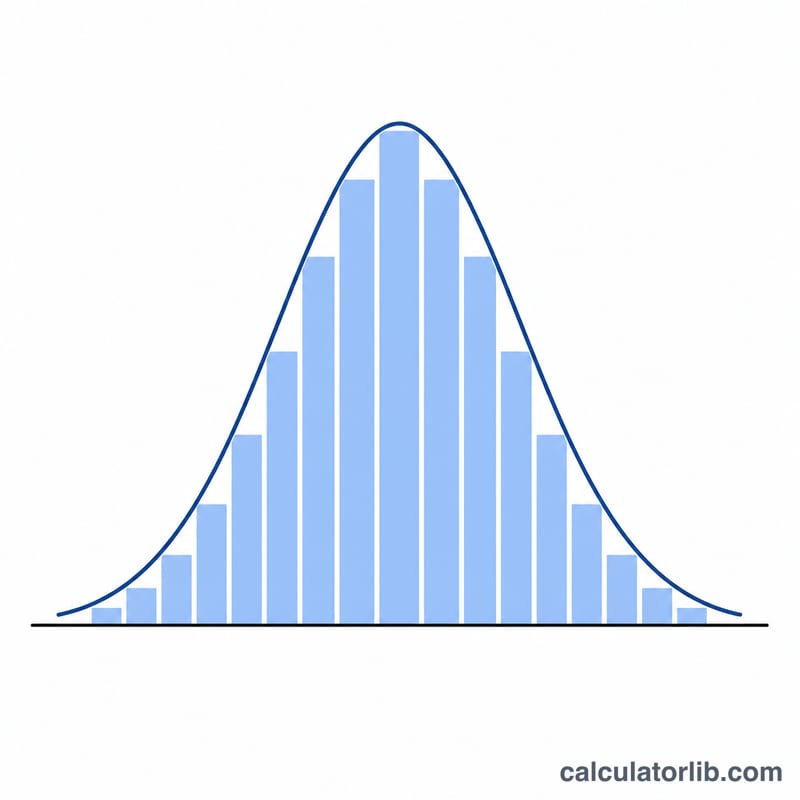
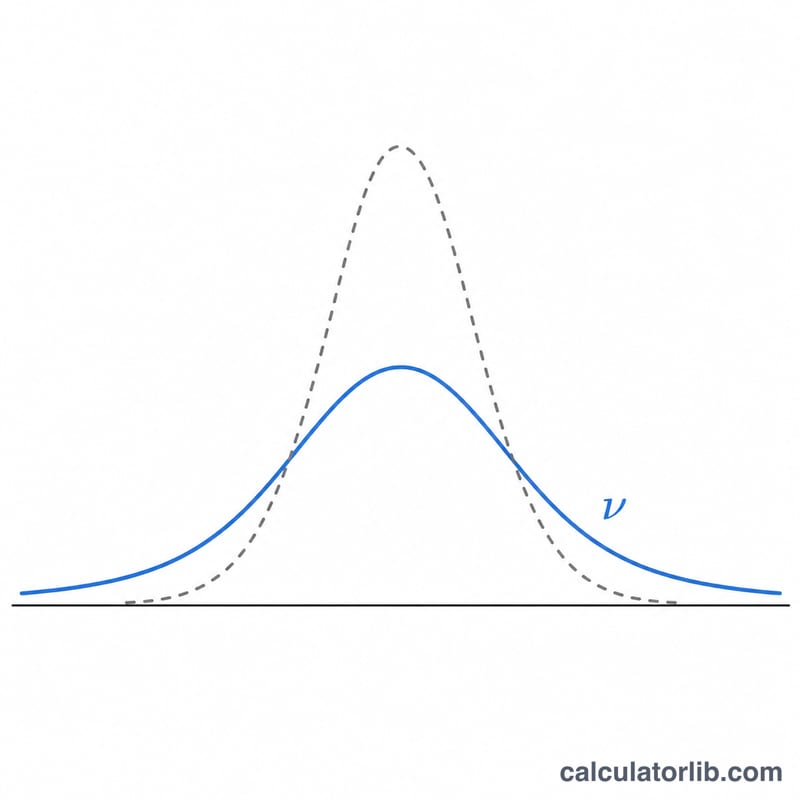
This generator produces a list of pseudo-random numbers drawn from a Student's t-distribution with a chosen number of degrees of freedom (v). The t-distribution is a bell-shaped, symmetric distribution that is heavier-tailed than the standard normal. It arises naturally when estimating the mean of a normally distributed population from a small sample with unknown variance, and it underpins the t-test and confidence intervals. As v grows large the t-distribution converges to the standard normal \(\mathcal{N}(0,1)\). This is a pure-mathematics tool with no regional assumptions.
How to use it
Enter the degrees of freedom v (any real number greater than 0; the default is 2) and the number of random values you want (an integer from 1 to 1000; the default is 10). Press calculate and a fresh list of t-distributed draws is returned. Because the underlying uniform draws are random, you get different numbers on every run, but they always follow the same target distribution.
The formula explained
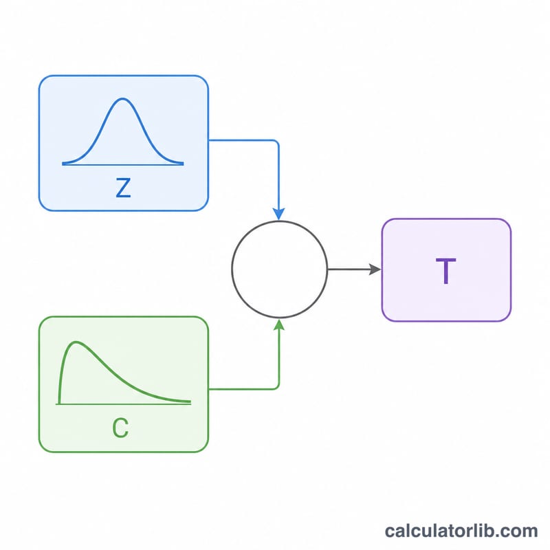
The density is \(f(x,v) = \dfrac{\left(1 + x^{2}/v\right)^{-(v+1)/2}}{\sqrt{v}\,B\!\left(\tfrac{1}{2}, \tfrac{v}{2}\right)}\), where \(B\) is the Beta function. To sample efficiently we use the classic representation: draw \(Z\) from a standard normal and \(C\) from a chi-square with v degrees of freedom, then $$T = Z \cdot \sqrt{\frac{v}{C}}$$ is exactly t-distributed. Internally \(Z\) comes from the Box-Muller transform and \(C\) from a \(\text{Gamma}(v/2, 2)\) sampler (Marsaglia-Tsang), valid for any real \(v > 0\).
Worked example
With v = 2, suppose one run gives \(Z = 0.50\) and a chi-square draw \(C = 1.20\). Then $$T = 0.50 \cdot \sqrt{\frac{2}{1.20}} = 0.50 \cdot 1.29099 = 0.6455.$$ A second pair \(Z = -1.10\), \(C = 3.00\) gives \(T = -0.8982\), and a third \(Z = 0.20\), \(C = 0.40\) gives \(T = 0.4472\). These three values illustrate a sample for count = 3.
FAQ
Why are some values huge? For \(v \le 1\) the mean is undefined and for \(v \le 2\) the variance is infinite, so large-magnitude draws are expected, not errors.
Why do results change each run? Each draw uses fresh random uniforms, so the list differs every time while still following the t-distribution.
What if v is very large? The distribution behaves almost identically to a standard normal \(\mathcal{N}(0,1)\).


