What this tool does
This generator produces a list of pseudo-random numbers that follow a normal (Gaussian) distribution with a mean and standard deviation that you choose. It uses the classic Box-Muller transform, a simple and exact method for turning uniformly distributed random numbers into normally distributed ones. The output is the core deliverable: a comma-separated list of values, each drawn from N(μ, σ²).
How to use it
Enter the mean (μ) — the center of the distribution — and the standard deviation (σ) — how spread out the values should be. Set how many numbers you want (1 to 1000) and pick a display precision in significant digits. Each run is stochastic, so you will get a fresh set of numbers every time you submit.
The formula explained
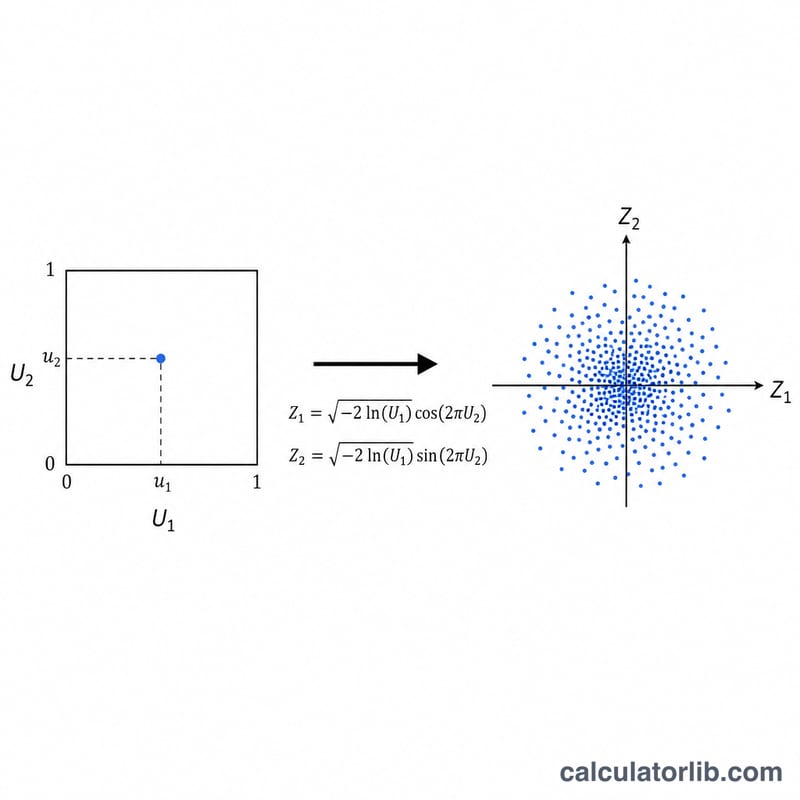
Draw two independent uniform numbers U1 and U2 on the open interval (0,1). The Box-Muller transform converts them into two independent standard-normal variates: Z1 = √(−2·ln U1)·cos(2πU2) and Z2 = √(−2·ln U1)·sin(2πU2). Each pass therefore yields two normals at once. We rescale each standard normal with X = μ + σ·Z. To avoid ln(0) = −∞, U1 is guarded so it is never exactly zero.
Worked example
Let μ = 100, σ = 15, and suppose U1 = 0.5, U2 = 0.25. Then √(−2·ln 0.5) = √1.386294 = 1.177410. With cos(π/2) = 0 and sin(π/2) = 1, we get Z1 = 0 and Z2 = 1.177410. So X1 = 100 + 15·0 = 100 and X2 = 100 + 15·1.177410 = 117.66115. Over many pairs the set's sample mean approaches 100 and its sample standard deviation approaches 15.
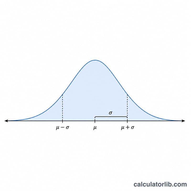
The 68-95-99.7 Rule (Empirical Rule)
For any normal distribution \(N(\mu, \sigma^2)\), a predictable share of values falls within a fixed number of standard deviations of the mean. This is the empirical rule, and it is a useful sanity check for the numbers you generate: with a large enough sample, the proportions below should emerge automatically.
| Interval | Value range | Proportion inside | Proportion in the tails |
|---|---|---|---|
| \(\pm 1\sigma\) | \(\mu - \sigma\) to \(\mu + \sigma\) | 68.27% | 31.73% |
| \(\pm 2\sigma\) | \(\mu - 2\sigma\) to \(\mu + 2\sigma\) | 95.45% | 4.55% |
| \(\pm 3\sigma\) | \(\mu - 3\sigma\) to \(\mu + 3\sigma\) | 99.73% | 0.27% |
Example: if you generate numbers with \(\mu = 100\) and \(\sigma = 15\), then about 68% of values should land between 85 and 115, about 95% between 70 and 130, and about 99.7% between 55 and 145. Values outside \(\pm 3\sigma\) (below 55 or above 145 here) are expected only about 3 times in 1,000 draws.
Interpreting Your Generated Numbers
The Box-Muller transform produces values that follow a normal (Gaussian) distribution centered on your chosen mean \(\mu\) with spread set by your standard deviation \(\sigma\). Read them with these facts in mind:
- Most values cluster near the mean. The bell shape is densest at \(\mu\), so a typical draw is close to \(\mu\); roughly two-thirds of values fall within one \(\sigma\) of it.
- Extreme values are rare but possible. A value far out in a tail (say beyond \(3\sigma\)) is unusual, not impossible — it occurs about 0.27% of the time. Seeing an occasional outlier is normal behavior, not a bug.
- Sample statistics converge as \(n\) grows. For a small count the sample mean and sample standard deviation can differ noticeably from \(\mu\) and \(\sigma\) by chance. As you increase
count, the sample mean approaches \(\mu\) and the sample SD approaches \(\sigma\) (law of large numbers). You can paste a batch into a Sample Mean Calculator or a Population Standard Deviation Calculator to confirm the values drift toward your targets. - This is for simulation and testing. These are pseudo-random draws meant for Monte Carlo experiments, load/stress testing, teaching, and modeling — not actual measurements of any real-world quantity. The numbers carry no empirical meaning beyond the distribution you specified.
Definitions & Glossary
- Mean (\(\mu\))
- The center, or expected value, of the distribution — the average around which generated values are balanced.
- Standard deviation (\(\sigma\))
- A measure of spread in the same units as the data. Larger \(\sigma\) produces values scattered more widely from the mean.
- Variance (\(\sigma^2\))
- The square of the standard deviation, \(\sigma^2\). It quantifies spread in squared units and is the parameter that appears in the distribution notation \(N(\mu, \sigma^2)\).
- Standard normal, \(N(0,1)\)
- The special normal distribution with mean 0 and standard deviation 1. Any value \(Z\) drawn from it is rescaled to your distribution via \(X = \mu + \sigma Z\).
- Uniform distribution
- A distribution in which every value in an interval (here, \((0,1)\)) is equally likely. The Box-Muller method starts from two independent uniform draws \(U_1\) and \(U_2\).
- Z-score
- The signed number of standard deviations a value lies from the mean, \(Z = (X - \mu)/\sigma\). A Z-score of 0 is exactly at the mean; \(\pm 2\) marks the edge of the central 95.45%.
- Pseudo-random
- Generated by a deterministic algorithm that produces sequences with the statistical properties of randomness. The output looks random and passes statistical tests but is fully reproducible from the same seed.
- Box-Muller transform
- A method that converts two independent uniform random numbers \(U_1, U_2\) into a standard normal value using \(Z = \sqrt{-2\ln U_1}\,\cos(2\pi U_2)\), which is then shifted and scaled to the requested mean and standard deviation.
FAQ
Why do the numbers change every time? The generator uses fresh uniform draws with no fixed seed, so output is random by design.
What if I set σ = 0? The distribution is degenerate and every generated value equals the mean.
Why does my sample mean not exactly equal μ? Random sampling produces sampling error; the more numbers you generate, the closer the sample mean and standard deviation get to μ and σ.


