What this generator does
This tool produces a list of pseudo-random numbers that follow a log-normal distribution. A random variable X is log-normal when its natural logarithm, \(\ln(X)\), is normally distributed. The generator first creates standard-normal variates with the classic Box-Muller transform, scales them to the target normal \(N(\mu, \sigma^2)\), and then exponentiates to obtain strictly positive log-normal values.
Important: what mu and sigma mean
The parameters \(\mu\) and \(\sigma\) describe the underlying normal distribution of \(\ln(X)\) — they are not the mean and standard deviation of X itself. The actual mean of X is \(\exp(\mu + \sigma^2/2)\), the median is \(\exp(\mu)\), and the variance is \((\exp(\sigma^2) - 1)\cdot\exp(2\mu + \sigma^2)\). These reference values are shown alongside your sample so you can sanity-check the output.
$$\begin{aligned} \text{Mean} &= \exp\!\left(\mu + \tfrac{1}{2}\sigma^{2}\right) \\ \text{Median} &= \exp\!\left(\mu\right) \\ \text{Var} &= \left(e^{\sigma^{2}} - 1\right) e^{\,2\mu + \sigma^{2}} \end{aligned}$$How to use it
Enter \(\mu\) (any real number), \(\sigma\) (zero or positive), and how many numbers you want (1 to 1000). Pick how many significant digits to display. Each run draws fresh uniform random numbers, so the values change every time. Because the Box-Muller method yields two normal variates per uniform pair, an odd count simply discards one spare variate.
The formula explained
For uniforms \(U_1, U_2\) in \((0,1]\):
$$X = \exp\!\left(\mu + \sigma\, Z\right), \quad Z = \sqrt{-2\ln U_1}\,\cos(2\pi U_2)$$\(Z = \sqrt{-2\cdot\ln U_1}\cdot\cos(2\pi\cdot U_2)\) gives \(Z \sim N(0,1)\). Then \(Y = \mu + \sigma\cdot Z\) is \(N(\mu, \sigma^2)\), and \(X = \exp(Y)\) is log-normal. We guard against \(\ln(0)\) by clamping \(U_1\) to a tiny epsilon.
$$\begin{gathered} X = \exp\!\left(\mu + \sigma\, Z\right) \\[1.5em] \text{where}\quad \left\{ \begin{aligned} Z &= \sqrt{-2\ln U_1}\,\cos(2\pi U_2) \\ U_1, U_2 &\sim \text{Uniform}(0,1) \end{aligned} \right. \end{gathered}$$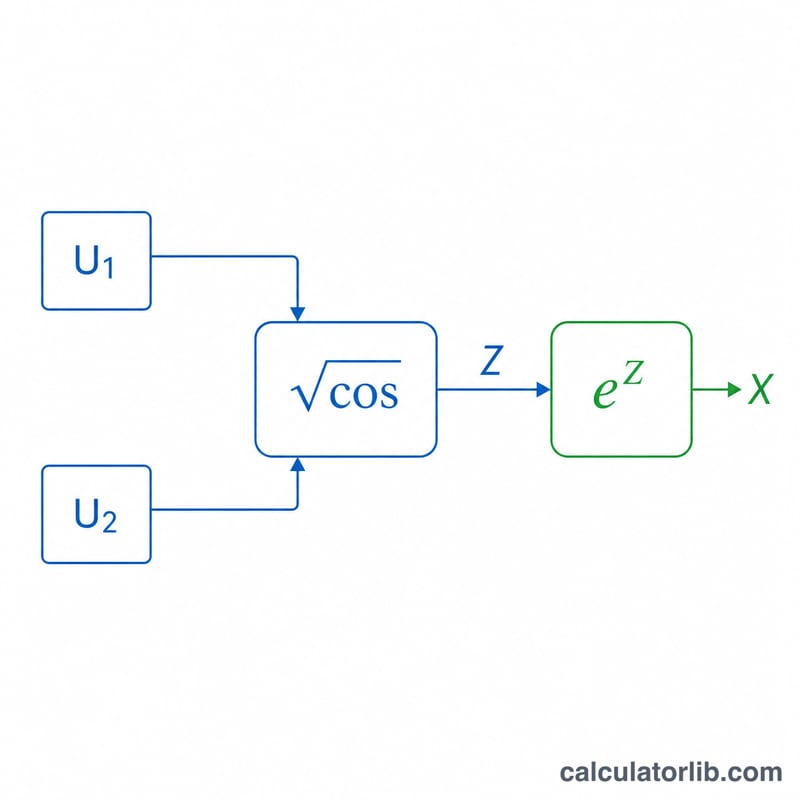
Worked example
With \(\mu = 1\), \(\sigma = 2\), take \(U_1 = 0.5\), \(U_2 = 0.25\). Then \(R = \sqrt{-2\cdot\ln 0.5} = 1.17741\). \(Z_1 = R\cdot\cos(\pi/2) = 0\) and \(Z_2 = R\cdot\sin(\pi/2) = 1.17741\). So
$$X_1 = \exp(1) = 2.71828$$and
$$X_2 = \exp(1 + 2\cdot 1.17741) = \exp(3.35482) \approx 28.64$$The theoretical mean \(\exp(3) = 20.0855\) and median \(\exp(1) = 2.71828\) are consistent.
FAQ
Why are my values different each run? It is a stochastic generator using Math.random(); without a fixed seed each run differs.
What if sigma = 0? The distribution is degenerate and every value equals \(\exp(\mu)\).
Can a value be negative? No — log-normal support is \((0, \infty)\), so all outputs are strictly positive.


