What is the log-normal distribution?
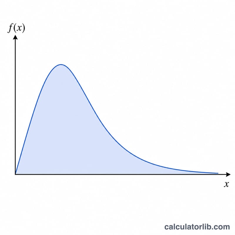
A positive random variable X is log-normally distributed when its natural logarithm ln(X) follows a normal distribution. In other words, X = e^Y where Y is Normal with mean mu and standard deviation sigma. Because logarithms are only defined for positive values, the log-normal distribution lives entirely on the positive real numbers, which makes it a natural model for quantities that cannot be negative: stock prices, income, particle sizes, biological measurements and time-to-failure data.
How to use this calculator
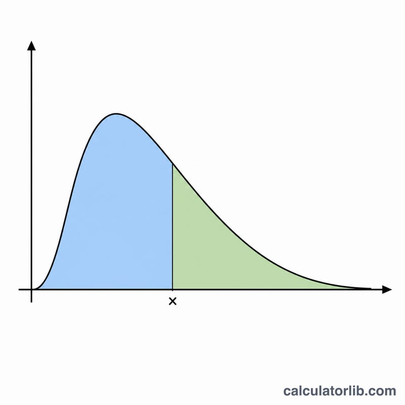
Enter the value x at which you want to evaluate the distribution (it must be greater than 0), then enter mu and sigma. A key point that trips up beginners: mu and sigma here are the mean and standard deviation of ln(X), not of X itself. The calculator returns three numbers: the probability density \(f(x)\), the lower cumulative probability \(P(x) = P(X \le x)\), and the upper cumulative probability \(Q(x) = P(X > x) = 1 - P(x)\).
The formula explained
Define the standardized score \(z = (\ln x - \mu) / \sigma\). The density is $$f(x) = \frac{1}{x\cdot\sigma\cdot\sqrt{2\pi}}\cdot\exp\!\left(-\frac{z^2}{2}\right)$$ The lower cumulative probability is \(P(x) = \Phi(z)\), where \(\Phi\) is the standard normal cumulative distribution function, $$\Phi(z) = 0.5\cdot\left(1 + \operatorname{erf}\!\left(\frac{z}{\sqrt{2}}\right)\right)$$ Since erf is not built into standard math libraries, this tool uses the Abramowitz & Stegun 7.1.26 polynomial approximation, which is accurate to about \(1.5 \times 10^{-7}\).
Worked example
Take \(x = 2\), \(\mu = 0\), \(\sigma = 1\). Then \(\ln(2) = 0.693147\) and \(z = 0.693147\). The density is $$f(2) = \frac{0.786429}{5.013256} \approx 0.156874$$ The lower cumulative probability is \(\Phi(0.693147) \approx 0.755891\), so the upper cumulative probability is $$Q(2) = 1 - 0.755891 \approx 0.244109$$
FAQ
Why must x be positive? The log-normal distribution is defined only for \(x > 0\) because \(\ln(x)\) is undefined otherwise. For \(x \le 0\) the density is 0, \(P(x) = 0\) and \(Q(x) = 1\).
How do I get the mean of X itself? The mean of X equals \(\exp(\mu + \sigma^2/2)\), the median equals \(\exp(\mu)\), and the mode equals \(\exp(\mu - \sigma^2)\). Note these differ from mu and sigma, which describe ln(X).
What if sigma is 0? A zero standard deviation gives a degenerate point mass and divides by zero, so it is rejected; use a small positive sigma instead.


