What this calculator does
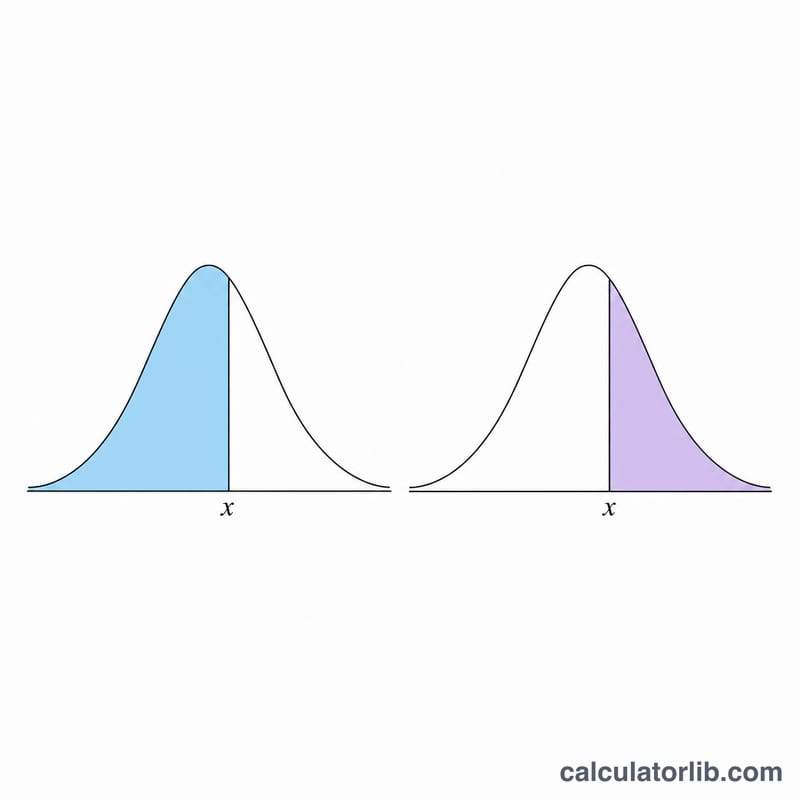
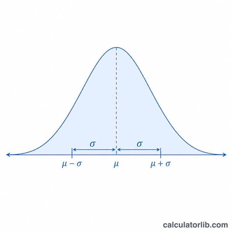
The Normal Distribution Graph Calculator builds a table of (x, value) pairs for the normal (Gaussian) distribution. You choose one of three functions to tabulate: the probability density \(f(x)\), the lower cumulative probability \(P(x)\) (the cumulative distribution function, or CDF), or the upper cumulative probability \(Q(x)\) (the survival function). The series of x values is defined by an initial value, a step (increment), and the number of points to generate. With mean \(\mu = 0\) and standard deviation \(\sigma = 1\) you get the standard normal distribution.
How to use it
Pick a function. Enter the mean \(\mu\) and the standard deviation \(\sigma\) (which must be greater than 0). Set the initial value of x, the increment between consecutive x values, and the number of repetitions (points). The calculator outputs a table where each row i gives \(x = \text{initialX} + i \cdot \text{step}\) and the chosen function evaluated at that x. The default settings (\(\mu=0\), \(\sigma=1\), start = -5, step = 0.1, 101 points) sweep x from -5 to +5 and trace the familiar bell curve for f or the S-shaped curve for P.
The formula explained
The density is $$f(x,\mu,\sigma) = \frac{1}{\sigma\sqrt{2\pi}}\, e^{-\frac{1}{2}\left(\frac{x - \mu}{\sigma}\right)^{2}}.$$ The cumulative probabilities use the error function: with \(z = \frac{x-\mu}{\sigma\sqrt{2}}\), the lower cumulative is $$P = \frac{1}{2}\left(1 + \operatorname{erf} z\right)$$ and the upper cumulative is \(Q = 1 - P\). Because Java/Groovy has no built-in erf, this tool uses the Abramowitz & Stegun 7.1.26 polynomial approximation, accurate to about \(1.5\times10^{-7}\).
Worked example
Standard normal (\(\mu=0\), \(\sigma=1\)) at x = 1: $$f(1) = 0.3989423 \cdot e^{-0.5} = 0.241971.$$ For P, \(z = \frac{1}{\sqrt{2}} = 0.70711\), \(\operatorname{erf}(z) \approx 0.68269\), so $$P = \frac{1}{2}(1 + 0.68269) = 0.84134$$ (the well-known \(\Phi(1) \approx 0.8413\)). Then \(Q = 1 - 0.84134 = 0.15866\), and \(P + Q = 1\). ✓
FAQ
Why must \(\sigma\) be positive? A zero or negative standard deviation has no meaning and would divide by zero in the formulas, so the tool rejects it.
Can the step be negative? Yes. A negative step counts x downward; a zero step gives a constant column of identical x values.
How accurate are P and Q? They use a polynomial erf approximation with maximum error around \(1.5\times10^{-7}\), more than enough for graphing and most statistical work.


