What is the noncentral F-distribution?
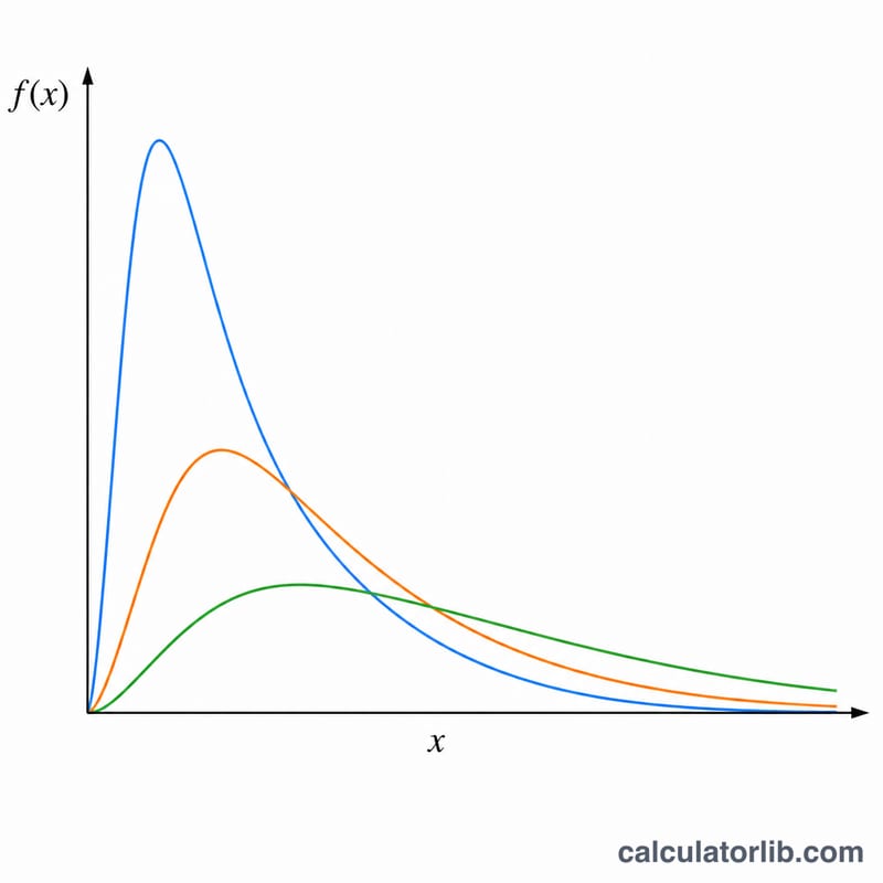
The noncentral F-distribution generalizes the ordinary (central) F-distribution by adding a noncentrality parameter lambda. It arises as the distribution of the ratio of a noncentral chi-square variate (divided by its degrees of freedom nu1) to an independent central chi-square variate (divided by nu2). It is fundamental to statistical power analysis: when a null hypothesis is false, the test statistic of an ANOVA or regression F-test follows a noncentral F, and lambda measures how far from the null the true effect lies. When \(\lambda = 0\) the distribution collapses to the familiar central F-distribution.
How to use this calculator
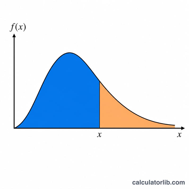
Choose which quantity to compute: the probability density f, the lower cumulative probability P (the CDF, area to the left of x), or the upper cumulative probability \(Q = 1 - P\) (area to the right). Enter the numerator degrees of freedom \(\nu_1\), the denominator degrees of freedom \(\nu_2\), and the noncentrality \(\lambda\). Then define a series of x values with an initial value, an increment (step) and a number of repetitions; the tool evaluates the selected function at \(x = \text{initialX} + i \cdot \text{step}\) for \(i = 0..\text{count}-1\) and tabulates the result.
The formula explained
The density is a Poisson-weighted average of central F densities. Each weight is $$w_j = \frac{e^{-\lambda/2}\left(\lambda/2\right)^{j}}{j!},$$ the probability of j events in a Poisson with mean \(\lambda/2\). The j-th term is the central F density with degrees of freedom \((\nu_1 + 2j,\ \nu_2)\), written with the Beta function $$B(a,b) = \frac{\Gamma(a)\Gamma(b)}{\Gamma(a+b)}.$$ The cumulative probability replaces each density by the corresponding central F CDF, which equals the regularized incomplete Beta function \(I_z\!\left(\tfrac{\nu_j}{2}, \tfrac{\nu_2}{2}\right)\) evaluated at $$z = \frac{\nu_j\,x}{\nu_2 + \nu_j\,x}.$$
Worked example
Take \(\nu_1 = 3\), \(\nu_2 = 2\), \(\lambda = 0\) (central case) and find P at \(x = 1\). Then $$z = \frac{3 \cdot 1}{2 + 3 \cdot 1} = 0.6$$ and \(P = I_{0.6}(1.5, 1.0)\). Since \(I_z(a,1) = z^a\), this is $$0.6^{1.5} = 0.464758,$$ so P approximately 0.4648 and Q approximately 0.5352. Adding noncentrality \(\lambda = 1\) shifts mass toward larger x, lowering the lower probability to about \(P = 0.451\).
FAQ
What happens when \(\lambda = 0\)? The result is exactly the central F-distribution: only the \(j = 0\) term carries weight.
Why is the density zero at \(x = 0\)? For \(\nu_1 \geq 2\) the density is 0 at \(x = 0\); for \(\nu_1 < 2\) it diverges to infinity as x approaches 0, so a value at \(x = 0\) is not meaningful there.
How accurate is the series? The Poisson weights are summed until the cumulative mass is essentially 1, and the incomplete Beta function is evaluated by a continued fraction with log-gamma for stability, giving high precision across typical inputs.


