What is the Binomial Distribution Calculator?
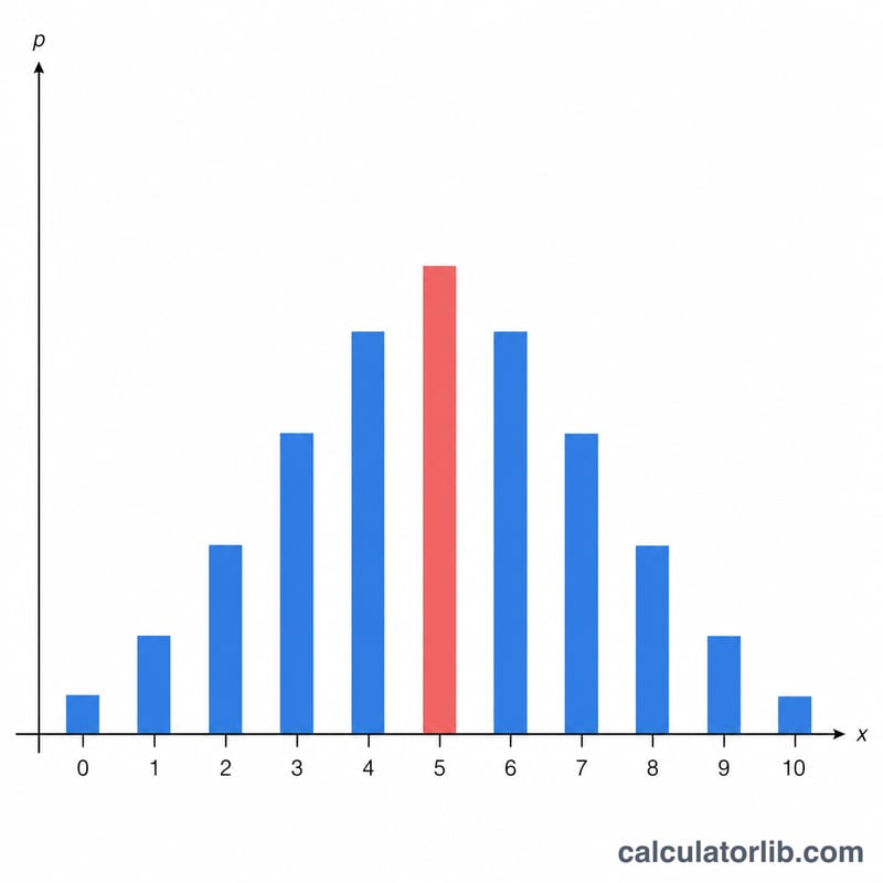
This tool evaluates the binomial distribution for a fixed number of independent trials. Given the number of successes x, the number of trials n, and the single-trial success probability p, it returns the probability of exactly x successes (the probability mass), the lower cumulative probability, the upper cumulative probability, and the mean. The binomial model applies whenever you repeat the same yes/no experiment a fixed number of times with a constant success chance, such as coin flips, defective parts in a batch, or quiz questions answered correctly by guessing.
How to use it
Enter three pure numbers. The successes x and trials n must be whole numbers with 0 ≤ x ≤ n and n ≥ 1. The probability p must be between 0 and 1. Press calculate to get all four outputs at once. Note this is a discrete distribution, so the headline figure is a probability mass (a true probability), not a probability density.
The formula explained
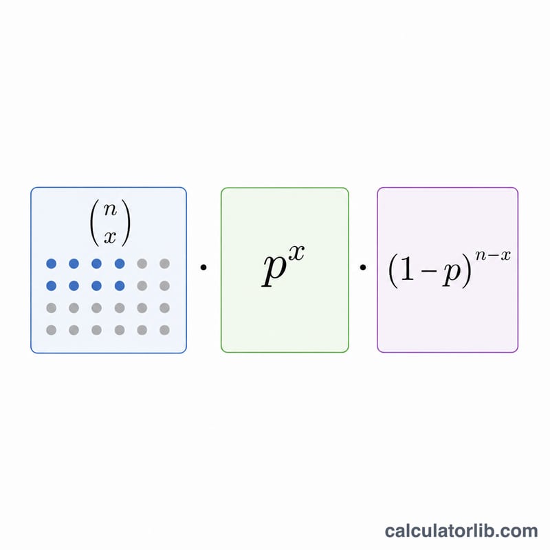
The probability mass is $$f(x,n,p) = \binom{n}{x} \cdot p^{x} \cdot (1-p)^{n-x},$$ where \(\binom{n}{x} = n! / (x!(n-x)!)\) is the binomial coefficient counting how many ways x successes can occur among n trials. The lower cumulative probability \(P(X \le x)\) sums \(f(t)\) for t from 0 to x, and the upper cumulative \(Q(X \ge x)\) sums \(f(t)\) for t from x to n. Because the point \(t=x\) is included in both sums, \(P + Q - f(x) = 1\). The mean is simply \(\mu = n \cdot p\). Coefficients are computed with log-factorials to stay stable for large n.
Worked example
For \(x = 9\), \(n = 20\), \(p = 0.4\): \(\binom{20}{9} = 167960\), \(p^{9} = 0.000262144\), and \(0.6^{11} \approx 0.0036279706\). So $$f = 167960 \times 0.000262144 \times 0.0036279706 \approx 0.15974.$$ The mean is \(20 \times 0.4 = 8\). Summing gives \(P(X \le 9) \approx 0.75534\) and \(Q(X \ge 9) \approx 0.40440\), which satisfy \(0.75534 + 0.40440 - 0.15974 \approx 1\).
Definitions & Glossary
The binomial distribution models the number of successes in a fixed number of independent yes/no experiments. The terms below appear throughout this calculator.
- Trial: a single repetition of the experiment that results in one of two possible outcomes (e.g. one coin flip).
- Success: the outcome you are counting, whatever you define it to be (heads, a defective part, a correct guess). Its complement is a "failure."
- n (number of trials): the total number of independent trials performed. It must be a fixed positive integer.
- x (number of successes): the specific count of successes whose probability you want, where \(0 \le x \le n\).
- p (probability of success): the probability that any single trial is a success, a decimal between 0 and 1.
- q = 1 − p (probability of failure): the probability that a single trial is a failure.
- Binomial coefficient \(\binom{n}{x}\): the number of distinct ways to choose which \(x\) of the \(n\) trials are successes, computed as \(\binom{n}{x}=\dfrac{n!}{x!\,(n-x)!}\).
- Probability mass function (pmf), \(f(x)\): the probability of exactly \(x\) successes, \(f(x)=\binom{n}{x}p^{x}(1-p)^{n-x}\).
- Lower cumulative probability, \(P(X \le x)\): the probability of at most \(x\) successes, the sum of pmf values from 0 through \(x\).
- Upper cumulative probability, \(P(X \ge x)\): the probability of at least \(x\) successes, the sum of pmf values from \(x\) through \(n\).
- Mean (expected value), \(\mu = np\): the average number of successes expected over many repetitions.
- Variance, \(\sigma^{2}=np(1-p)\): the spread of the distribution around its mean.
- Standard deviation, \(\sigma=\sqrt{np(1-p)}\): the typical deviation of the success count from the mean, in the same units as \(x\).
Interpreting Your Result
This calculator returns three probabilities and the mean. Choose the one that matches the wording of your question:
- pmf, \(f(x)=P(X=x)\) — use when you want the chance of exactly \(x\) successes, e.g. "exactly 5 heads in 10 flips."
- Lower cumulative, \(P(X \le x)\) — use for at most \(x\) ("\(x\) or fewer"), e.g. "5 or fewer correct answers."
- Upper cumulative, \(P(X \ge x)\) — use for at least \(x\) ("\(x\) or more"), e.g. "at least 1 defective part."
Note the cumulative pieces overlap at \(x\): \(P(X \le x)+P(X \ge x)=1+f(x)\), because both ranges include the value \(x\) itself. To get strictly fewer than \(x\), use \(P(X \le x-1)\); for strictly more than \(x\), use \(P(X \ge x+1)\).
The mean \(np\) is the expected number of successes — the long-run average if you repeated the whole \(n\)-trial experiment many times. It need not be a whole number; an expected value of 4.5 simply describes an average.
All probabilities are reported as decimals between 0 and 1 (multiply by 100 for a percentage). A value near 0 means the event is rare; near 1, nearly certain.
These results are valid only when the four binomial assumptions hold:
- Fixed number of trials \(n\), decided before observing outcomes.
- Two outcomes per trial — each trial is a success or a failure.
- Constant probability \(p\) of success on every trial.
- Independence — the result of one trial does not affect any other.
If trials are not independent or \(p\) drifts between trials (for example, sampling without replacement from a small population), the binomial model is only an approximation.
FAQ
Is the upper cumulative inclusive of x? Yes. Here \(Q(X \ge x)\) includes the point \(t=x\), so it is \(P(X \ge x)\), not \(P(X > x)\).
What happens at p=0 or p=1? Using the \(0^{0}=1\) convention, \(p=0\) gives \(f(0)=1\) and all other probabilities 0; \(p=1\) gives \(f(n)=1\).
Why "probability mass" and not "density"? Density applies to continuous distributions; for a discrete variable each outcome carries an actual probability, so "mass" is the correct term.


