What this calculator does
The standard normal distribution N(0,1) is the bell curve with mean 0 and standard deviation 1. Given a percentage point x (also called a z-score), this calculator returns four numbers: the probability density at x, the lower cumulative probability P(X ≤ x), the upper cumulative probability P(X ≥ x), and the inner two-sided probability P(−|x| ≤ X ≤ |x|). It works for any real x, positive, negative, or zero.
How to use it
Enter a value for x and read off the results. For example, x = 1 corresponds to one standard deviation above the mean; x = 1.96 is the classic 95% confidence cutoff. The tool needs no units because the standard normal variable is dimensionless.
The formulas explained
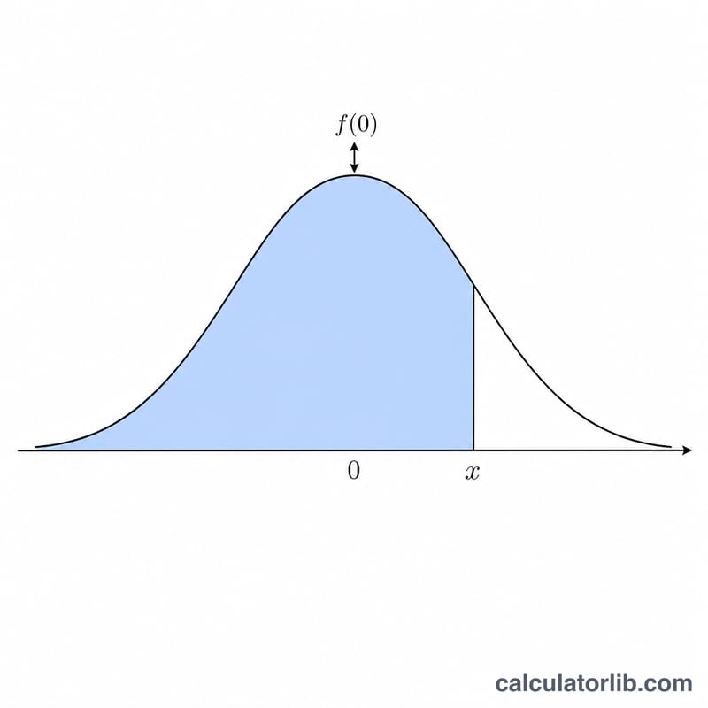
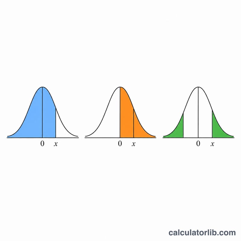
The density is $$\varphi(x) = \frac{1}{\sqrt{2\pi}}\, e^{-x^{2}/2}$$ where \(1/\sqrt{2\pi} \approx 0.3989423\). The lower cumulative distribution function is $$\Phi(x) = \frac{1}{2}\left[\,1 + \operatorname{erf}\!\left(\frac{x}{\sqrt{2}}\right)\right]$$ using the Gauss error function erf. The upper tail is \(Q(x) = 1 - \Phi(x)\), and the inner probability is \(I(x) = \operatorname{erf}(|x|/\sqrt{2}) = 2\Phi(|x|) - 1\). Because basic math libraries lack erf, we evaluate it with the Abramowitz & Stegun 7.1.26 rational approximation (maximum error about \(1.5\times10^{-7}\)), which is accurate to roughly six decimal places for display.
Worked example
For x = 1: $$\varphi(1) = 0.3989423 \times e^{-0.5} \approx 0.2419707$$ \(\operatorname{erf}(0.7071068) \approx 0.6826895\), so \(\Phi(1) \approx 0.8413447\), giving an upper tail of 0.1586553 and an inner probability of 0.6826895 — the familiar "68% of values fall within ±1 standard deviation."
FAQ
What is a z-score? It is the number of standard deviations a value lies from the mean. For the standard normal distribution the value and its z-score are the same.
Why does the inner probability use |x|? The two-sided region is symmetric about zero, so a negative x gives the same inner probability as its positive counterpart.
How accurate are the results? The error-function approximation is good to about six decimal places, which is more than enough for typical statistical work.


