Bivariate Standard Normal Distribution Calculator

Upper cumulative probability Q(x, y, ρ)	0.022035922476
Meaning	P(U1 > x and U2 > y)

What this calculator does

This tool evaluates the standard bivariate normal distribution, a two-dimensional Gaussian with zero means, unit variances on both axes, and a single free parameter: the correlation coefficient ρ. Given a point (x, y) it returns two numbers: the joint probability density $f(x, y, \rho)$ at that point, and the upper-tail (orthant) cumulative probability $Q(x, y, \rho) = P(U_1 > x \text{ AND } U_2 > y)$. Because every input is already a standardized, dimensionless score, the calculator is universal and needs no unit conversion.

3D bell-shaped surface of a bivariate normal density over the x-y plane — The joint density f(x,y) forms a bell-shaped surface over the x-y plane.

How to use it

Enter the percentile point x, the percentile point y, and the correlation ρ. Here "percentile point" means a z-like standardized threshold (a coordinate), not a 0-1 percentile. The correlation must satisfy $-1 < \rho < 1$; the values $\pm 1$ are rejected because the density becomes singular (division by zero in $\sqrt{1-\rho^{2}}$).

The formulas explained

The density is the closed-form Gaussian shown above:

$$\varphi(x,y;\rho) = \frac{1}{2\pi\sqrt{1-\rho^{2}}}\,\exp\!\left(-\frac{x^{2}-2\rho\,x\,y+y^{2}}{2\left(1-\rho^{2}\right)}\right)$$

The orthant probability uses Sheppard's identity: when $\rho = 0$ the variables are independent and $Q = Q_1(x)\cdot Q_1(y)$, where $Q_1(t)$ is the univariate upper-tail standard normal function. For nonzero $\rho$ we add a correction integral from 0 to $\rho$, evaluated here with 24-node Gauss–Legendre quadrature for accuracy.

$$\begin{gathered} Q(x,y;\rho) = Q_1(x)\,Q_1(y) + \frac{1}{2\pi}\int_{0}^{\rho}\frac{\exp\!\left(-\dfrac{x^{2}-2r\,x\,y+y^{2}}{2(1-r^{2})}\right)}{\sqrt{1-r^{2}}}\,dr \\[1.5em] \text{where}\quad \left\{ \begin{aligned} x &= \text{Percentile point x} \\ y &= \text{Percentile point y} \\ \rho &= \text{Correlation }\rho \\ Q_1(t) &= \tfrac{1}{2}\,\operatorname{erfc}\!\left(\tfrac{t}{\sqrt{2}}\right) \end{aligned} \right. \end{gathered}$$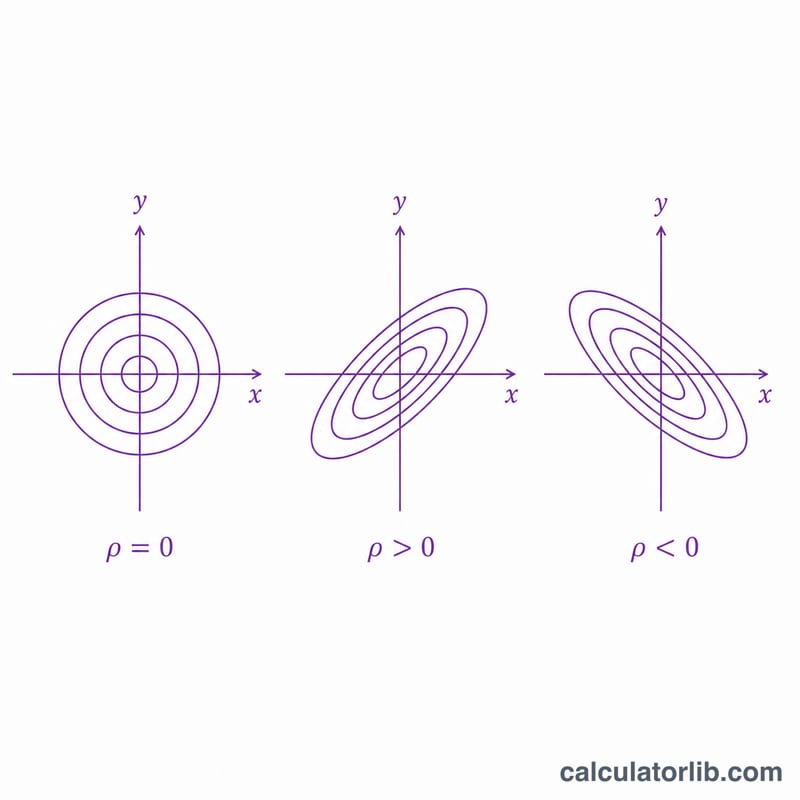

Three contour plots showing circular, positively tilted, and negatively tilted ellipses for different correlations — Elliptical density contours rotate with the correlation rho: circular when rho=0, tilted for positive or negative rho.

Worked example

For $x = 2$, $y = 0.7$, $\rho = 0.8$: $1 - \rho^{2} = 0.36$, $\sqrt{\phantom{x}} = 0.6$, prefactor $= 1/(2\pi\cdot 0.6) = 0.265258$. Exponent numerator $= 4 - 2\cdot 0.8\cdot 2\cdot 0.7 + 0.49 = 2.25$, divided by 0.72 gives 3.125. So $f = 0.265258 \cdot e^{-3.125} \approx 0.011655$. The upper probability $Q \approx 0.0212$ — higher than the independence value 0.0055 because positive correlation pushes both variables up together.

How Correlation Changes the Orthant Probability

The orthant probability $Q(x,y;\rho)=P(U_1>x,\,U_2>y)$ measures the chance that two standard normal variables simultaneously exceed their thresholds. Holding the cut-points fixed at $x=1$ and $y=1$ and sweeping the correlation $\rho$ isolates the pure effect of dependence. When $\rho=0$ the variables are independent and $Q$ factors into the product of the two univariate upper tails, $Q_1(x)\,Q_1(y)$. For a standard normal, $Q_1(1)=P(U>1)\approx 0.158655$, so the independence benchmark is $0.158655^2\approx$ 1) for standard normal">0.158655$^2 = 0.025172$.

$\rho$	Density $f(1,1;\rho)$	Orthant $Q(1,1;\rho)$	Independence $Q_1(1)Q_1(1)$
$-0.8$	0.0476	0.0049	0.0252
$-0.4$	0.0780	0.0145	0.0252
$0$	0.0585	0.0252	0.0252
$0.4$	0.1063	0.0438	0.0252
$0.8$	0.2643	0.0826	0.0252

The pattern is monotone: positive correlation makes joint exceedance more likely (large values tend to occur together), so $Q$ rises above the independence value; negative correlation pulls the two variables in opposite directions, so joint exceedance becomes rarer and $Q$ falls below $Q_1 Q_1$. At $\rho=0$ the orthant probability exactly equals the product $0.0252$, confirming the independence factorization.

Interpreting the Density and Orthant Probability

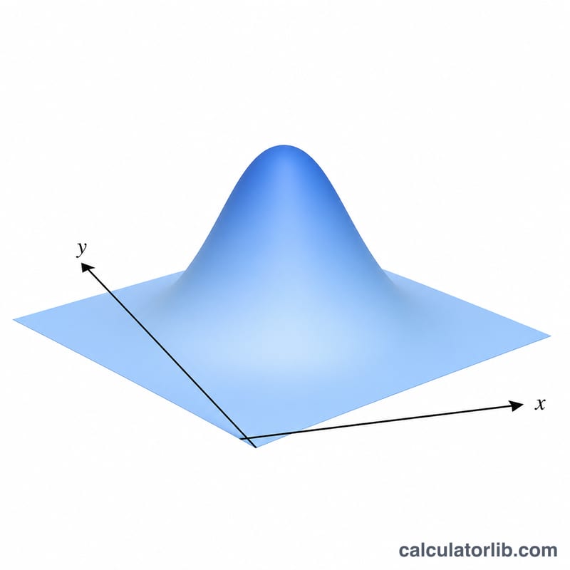
The density $f$ is not a probability. The value $\varphi(x,y;\rho)$ is a probability density per unit area in the $(x,y)$ plane; only its integral over a region returns a probability. The surface attains its maximum at the origin $(0,0)$, where the exponential term equals 1 and

$$f(0,0;\rho)=\frac{1}{2\pi\sqrt{1-\rho^{2}}}.$$

For $\rho=0$ this peak is $1/(2\pi)\approx 0.159$, comfortably below 1. As $\rho\to\pm 1$ the factor $1/\sqrt{1-\rho^2}$ diverges, so the peak density can exceed 1 — that is normal for a density, since it concentrates probability mass onto the line $y=\rho x$.

The orthant probability $Q$ is a genuine probability and always lies in $[0,1]$. It is the volume under the density surface over the quadrant $\{U_1>x,\,U_2>y\}$. Useful structural facts:

Independence ($\rho=0$): $Q(x,y;0)=Q_1(x)\,Q_1(y)$, the product of the two univariate upper tails.
Symmetry in arguments: by exchanging the roles of the two coordinates, $Q(x,y;\rho)=Q(y,x;\rho)$.
Reflection identity: $Q(-x,-y;\rho)=Q(x,y;\rho)+ \Phi(-x)+\Phi(-y)-1$ (equivalently expressible through the bivariate CDF), and reversing the sign of one argument flips the effective correlation: \(P(U_1>x,\,U_2
Limiting behavior $\rho\to 1^{-}$: the variables become perfectly comonotone, $U_2\approx U_1$, so $Q(x,y;\rho)\to Q_1(\max(x,y))$ — both exceedances coincide.
Limiting behavior $\rho\to -1^{+}$: the variables become perfectly countermonotone, $U_2\approx -U_1$. Joint upper exceedance is then possible only when both thresholds can be cleared simultaneously, giving $Q\to\max\!\big(0,\;1-\Phi(x)-\Phi(y)\big)$, which is 0 whenever $x+y\ge 0$.

Because there is no closed form for $Q$ with general $\rho$, it is evaluated numerically — typically through Owen's T function or a one-dimensional integral over $\rho$ using Gauss–Legendre quadrature, both of which reproduce the values shown in the comparison table to high precision.

Definitions & Glossary

Standardized score ($x$, $y$): A z-like coordinate measuring how many standard deviations a value sits from its mean. The inputs $x$ and $y$ are already standardized, so each marginally follows the standard normal $N(0,1)$ distribution.
Correlation coefficient $\rho$: The linear (Pearson) correlation between the two standard normal variables, with $-1<\rho<1$. It is the single parameter governing how strongly the two coordinates move together; $\rho=0$ means independence here, while $\rho\to\pm1$ means a near-deterministic linear relationship. An observed $\rho$ can be estimated from paired data with a Pearson correlation calculator.
Joint density $f(x,y;\rho)$: The standard bivariate normal probability density, $\varphi(x,y;\rho)=\dfrac{1}{2\pi\sqrt{1-\rho^2}}\exp\!\left(-\dfrac{x^2-2\rho xy+y^2}{2(1-\rho^2)}\right)$. It describes probability per unit area, not a probability itself.
Orthant probability $Q(x,y;\rho)$: The upper-tail joint probability $P(U_1>x,\,U_2>y)$ — the volume under the density surface over the upper-right quadrant defined by the two thresholds. Always between 0 and 1.
Univariate upper tail $Q_1(t)$: The standard normal survival function $Q_1(t)=P(U>t)=1-\Phi(t)$, the area in the right tail beyond $t$. For example $Q_1(1)\approx 0.1587$. At $\rho=0$, $Q=Q_1(x)Q_1(y)$.
Complementary error function ($\operatorname{erfc}$): A special function related to the normal tail by $Q_1(t)=\tfrac{1}{2}\operatorname{erfc}\!\left(t/\sqrt{2}\right)$. It provides a numerically stable way to compute the univariate tail probabilities used in $Q$.
Gauss–Legendre quadrature: A numerical integration scheme that approximates a definite integral by a weighted sum of the integrand at optimally chosen nodes. Because $Q(x,y;\rho)$ has no elementary closed form, it is commonly evaluated by integrating the density (or a function of $\rho$) with this method to obtain accurate results.

FAQ

Why can't ρ be exactly 1? At $\rho = \pm 1$ the two variables are perfectly dependent and the distribution collapses onto a line; the density has no finite value off that line.

What does Q represent? It is the probability mass in the upper-right "orthant" beyond both thresholds: $P(U_1 > x, U_2 > y)$.

What happens for large x or y? The density decays toward 0 and Q approaches 0, since it is increasingly unlikely both standardized variables exceed large positive thresholds.