What this calculator does
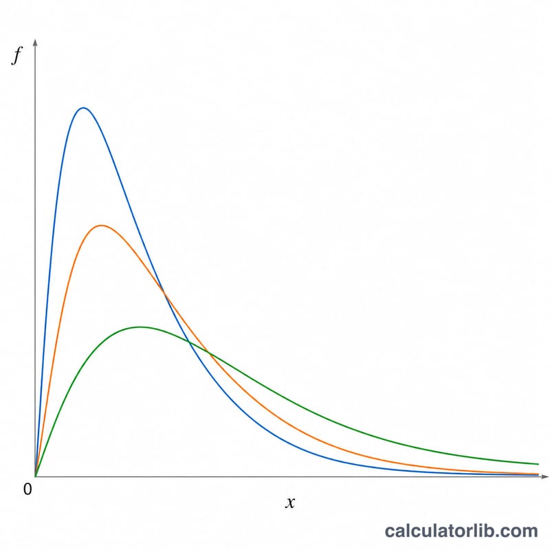
The F-distribution arises whenever you compare two variances, such as in ANOVA, regression overall-significance tests, and the F-test for equality of variances. This tool evaluates the F-distribution with numerator degrees of freedom \(\nu_1\) and denominator degrees of freedom \(\nu_2\) over a whole series of x values, so you can build a table and a graph in one step. Choose one of three functions: the probability density f, the lower cumulative probability P (the CDF), or the upper cumulative probability Q (the survival function, useful for right-tail p-values).
How to use it
Pick the function you want. Enter the two degrees of freedom (both must be greater than 0). Then set the series: the initial value of x (x must be >= 0), the increment between points, and the number of iterations. The calculator generates \(x_i = \text{initialX} + i \cdot \text{stepX}\) for \(i = 0\) to \(\text{loopCount}-1\) and reports the chosen function at each point. The default settings (\(\nu_1 = 3\), \(\nu_2 = 5\), start 0, step 0.1, 51 points) sweep x from 0 to 5.
The formula explained
The density uses the Beta function \(B(a,b) = \frac{\Gamma(a)\Gamma(b)}{\Gamma(a+b)}\). To stay numerically stable for large degrees of freedom we work in logarithms with the log-gamma function. The cumulative probability has a clean closed form:
$$F(x) = I_{\,z}\!\left(\tfrac{\nu_1}{2},\,\tfrac{\nu_2}{2}\right),\quad z = \frac{\nu_1 x}{\nu_1 x + \nu_2}$$where z = v1*x/(v1*x + v2). The upper tail is simply \(Q(x) = 1 - P(x)\). We evaluate the incomplete beta with the standard continued-fraction method. The density itself is
$$f(x) = \frac{\sqrt{\dfrac{(\nu_1 x)^{\nu_1}\,\nu_2^{\nu_2}}{(\nu_1 x + \nu_2)^{\nu_1+\nu_2}}}}{x\,B\!\left(\tfrac{\nu_1}{2},\tfrac{\nu_2}{2}\right)}$$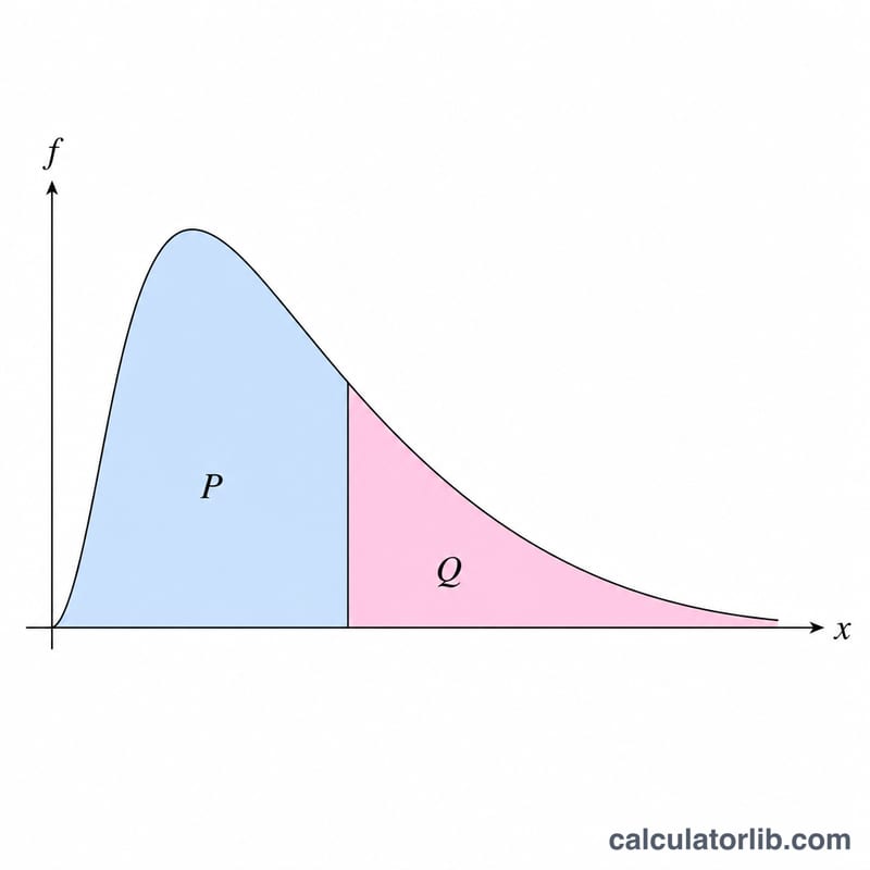
Worked example
With \(\nu_1 = 3\) and \(\nu_2 = 5\) at \(x = 1\): the constant
$$C = \frac{3^{1.5} \cdot 5^{2.5}}{B(1.5,\, 2.5)} = \frac{5.196152 \cdot 55.901699}{0.196350} = 1479.36$$Then
$$f = \frac{1479.36 \cdot 1^{0.5}}{(5 + 3)^4} = \frac{1479.36}{4096} = 0.36117$$For the CDF, \(z = 3/8 = 0.375\) gives
$$P = I_{0.375}(1.5,\, 2.5) = 0.5351,\quad \text{so } Q = 0.4649$$FAQ
Why does the density blow up at x = 0? When \(\nu_1 < 2\) the density is unbounded at \(x = 0\); at \(\nu_1 = 2\) it equals 1, and for \(\nu_1 > 2\) it is 0.
What range of x makes sense? The F variable is non-negative, so start at \(x = 0\) and extend far enough into the right tail (often x up to 5-10) to capture the bulk of the distribution.
Does the mean always exist? The mean \(\frac{\nu_2}{\nu_2-2}\) exists only for \(\nu_2 > 2\) and the variance only for \(\nu_2 > 4\), though neither is required to evaluate the functions here.


