通过MCP连接 →

输入计算

数学公式

广告

结果

Normal Distribution Table (f)
101
points generated · first value at x = -5: 0.00000149
x f(x)
-5 0.00000149
-4.9 0.00000244
-4.8 0.00000396
-4.7 0.00000637
-4.6 0.00001014
-4.5 0.00001598
-4.4 0.00002494
-4.3 0.00003854
-4.2 0.00005894
-4.1 0.00008926
-4 0.00013383
-3.9 0.00019866
-3.8 0.00029195
-3.7 0.00042478
-3.6 0.0006119
-3.5 0.00087268
-3.4 0.00123222
-3.3 0.00172257
-3.2 0.00238409
-3.1 0.00326682
-3 0.00443185
-2.9 0.00595253
-2.8 0.00791545
-2.7 0.01042093
-2.6 0.01358297
-2.5 0.0175283
-2.4 0.02239453
-2.3 0.02832704
-2.2 0.03547459
-2.1 0.0439836
-2 0.05399097
-1.9 0.06561581
-1.8 0.07895016
-1.7 0.09404908
-1.6 0.11092083
-1.5 0.1295176
-1.4 0.14972747
-1.3 0.17136859
-1.2 0.19418605
-1.1 0.21785218
-1 0.24197072
-0.9 0.26608525
-0.8 0.28969155
-0.7 0.31225393
-0.6 0.3332246
-0.5 0.35206533
-0.4 0.36827014
-0.3 0.38138782
-0.2 0.39104269
-0.1 0.39695255
0 0.39894228
0.1 0.39695255
0.2 0.39104269
0.3 0.38138782
0.4 0.36827014
0.5 0.35206533
0.6 0.3332246
0.7 0.31225393
0.8 0.28969155
0.9 0.26608525
1 0.24197072
1.1 0.21785218
1.2 0.19418605
1.3 0.17136859
1.4 0.14972747
1.5 0.1295176
1.6 0.11092083
1.7 0.09404908
1.8 0.07895016
1.9 0.06561581
2 0.05399097
2.1 0.0439836
2.2 0.03547459
2.3 0.02832704
2.4 0.02239453
2.5 0.0175283
2.6 0.01358297
2.7 0.01042093
2.8 0.00791545
2.9 0.00595253
3 0.00443185
3.1 0.00326682
3.2 0.00238409
3.3 0.00172257
3.4 0.00123222
3.5 0.00087268
3.6 0.0006119
3.7 0.00042478
3.8 0.00029195
3.9 0.00019866
4 0.00013383
4.1 0.00008926
4.2 0.00005894
4.3 0.00003854
4.4 0.00002494
4.5 0.00001598
4.6 0.00001014
4.7 0.00000637
4.8 0.00000396
4.9 0.00000244
5 0.00000149

这个计算器能做什么

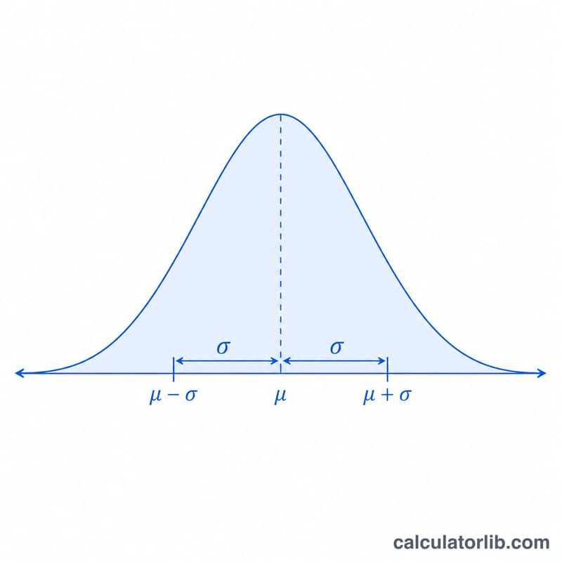
正态分布图计算器可以为正态(高斯)分布生成一张 (x, 数值) 对照表。你可以从三种函数中任选一种来制表:概率密度 \(f(x)\)、下侧累积概率 \(P(x)\)(即累积分布函数 CDF),或上侧累积概率 \(Q(x)\)(即生存函数)。x 的取值序列由初始值、步长(增量)和点数三项决定。当均值 \(\mu = 0\)、标准差 \(\sigma = 1\) 时,得到的就是标准正态分布。

Two bell curves showing left-shaded lower cumulative area P(x) and right-shaded upper cumulative area Q(x)
Lower cumulative P(x) is the shaded area to the left of x; upper cumulative Q(x) is the area to the right.

使用方法

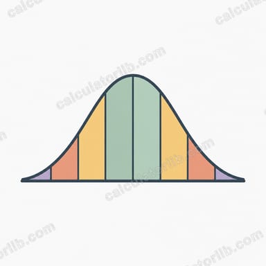
先选择一种函数。填入均值 \(\mu\) 和标准差 \(\sigma\)(\(\sigma\) 必须大于 0)。再设置 x 的初始值、相邻 x 之间的增量,以及重复次数(点数)。计算器会输出一张表格,其中第 i 行对应 \(x = \text{初始值} + i \cdot \text{步长}\),以及该 x 处所选函数的取值。默认设置(\(\mu=0\)、\(\sigma=1\)、起点 = -5、步长 = 0.1、共 101 个点)会让 x 从 -5 扫到 +5:选择 f 时描绘出我们熟悉的钟形曲线,选择 P 时则呈现出 S 形曲线。

公式详解

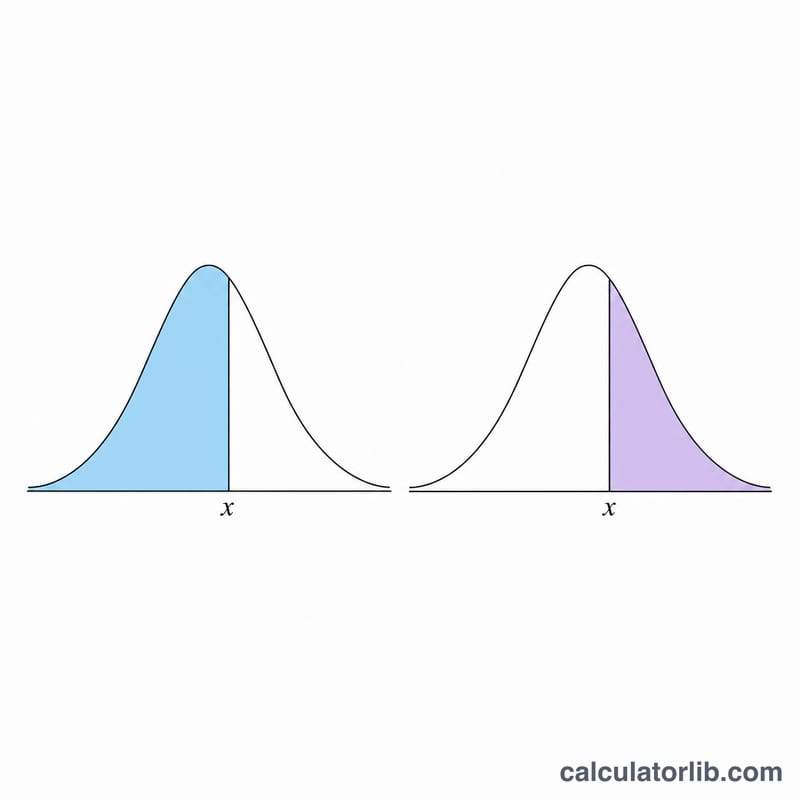
概率密度为 $$f(\text{x},\mu,\sigma) = \frac{1}{\sigma\sqrt{2\pi}}\, e^{-\frac{1}{2}\left(\frac{\text{x} - \mu}{\sigma}\right)^{2}}$$ 累积概率借助误差函数计算:令 \(z = \frac{\text{x}-\mu}{\sigma\sqrt{2}}\),则下侧累积概率 $$P = \frac{1}{2}\left(1 + \operatorname{erf} z\right)$$ 上侧累积概率 \(Q = 1 - P\)。由于 Java/Groovy 没有内置的 erf 函数,本工具采用 Abramowitz & Stegun 7.1.26 多项式近似公式,精度约为 \(1.5\times10^{-7}\)。

Advertisement
Bell-shaped normal distribution curve with mean mu at center and standard deviation sigma marked
The normal probability density f(x) forms a symmetric bell curve centered on the mean μ with spread set by σ.

实例演算

以标准正态分布(\(\mu=0\)、\(\sigma=1\))在 x = 1 处为例:$$f(1) = 0.3989423 \cdot e^{-0.5} = 0.241971$$ 计算 P 时,\(z = \frac{1}{\sqrt{2}} = 0.70711\),\(\operatorname{erf}(z) \approx 0.68269\),于是 $$P = \frac{1}{2}\left(1 + 0.68269\right) = 0.84134$$(即众所周知的 \(\Phi(1) \approx 0.8413\))。再求 \(Q = 1 - 0.84134 = 0.15866\),可见 \(P + Q = 1\)。✓

常见问题

为什么 \(\sigma\) 必须为正数?标准差为零或负数毫无意义,并且会在公式中导致除以零,因此本工具不接受这类输入。

步长可以是负数吗?可以。负步长会让 x 逐渐递减;步长为零则会得到一列完全相同的 x 值。

P 和 Q 的精度如何?二者采用多项式 erf 近似,最大误差约为 \(1.5\times10^{-7}\),对于绘图和绝大多数统计工作来说绰绰有余。

最后更新: