What this calculator does
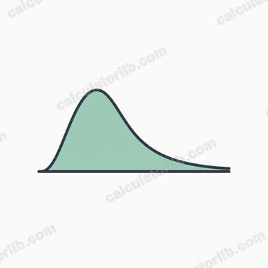
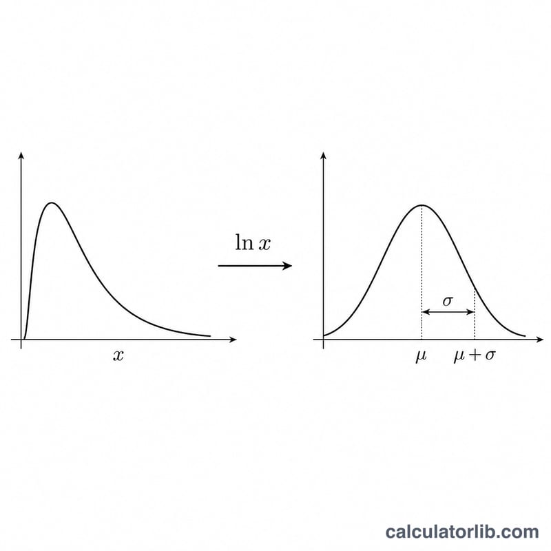
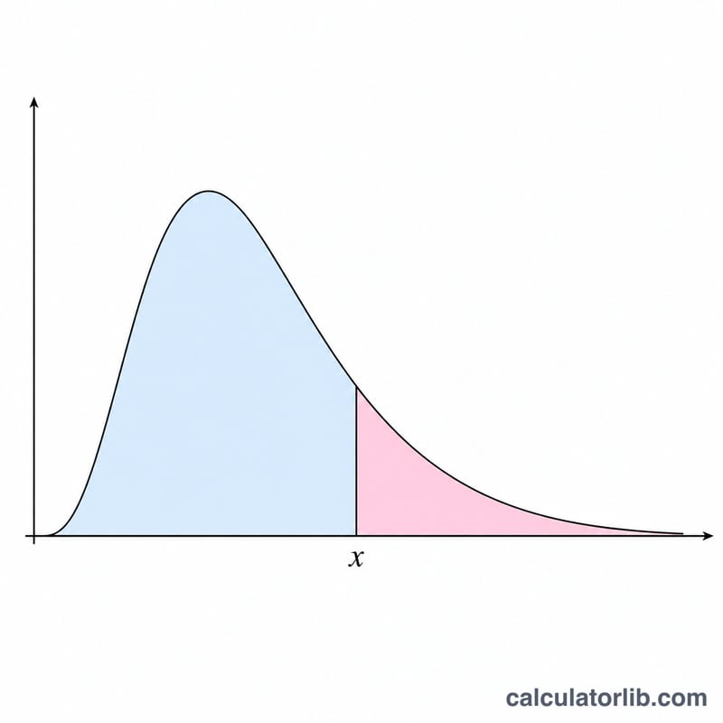
The lognormal distribution describes a positive random variable whose natural logarithm is normally distributed. If ln(x) follows a normal distribution with mean μ and standard deviation σ, then x is lognormally distributed. This calculator evaluates one of three functions over a chosen range of x values and returns a table you can read or plot: the probability density f(x), the lower cumulative probability P(x) (the cumulative distribution function), or the upper cumulative probability Q(x) = 1 − P(x).
How to use it
Pick the function to plot, then enter the mean μ and standard deviation σ of ln(x). Set the starting x (Initial value of x), the Step between successive x values, and the Number of points. The calculator evaluates the function at \(x_i = \text{initialX} + i \times \text{step}\) for \(i = 0, 1, \ldots, \text{count}-1\) and tabulates each (x, value) pair. Sigma must be positive and x must be non-negative; at x = 0 the density and lower cumulative are 0 while the upper cumulative is 1.
The formula explained
The density is $$f(x) = \frac{1}{x\,\sigma\sqrt{2\pi}}\exp\!\left(-\frac{\left(\ln x - \mu\right)^{2}}{2\,\sigma^{2}}\right),\quad x>0$$ The cumulative probability is $$P(x) = \Phi\!\left(\frac{\ln x - \mu}{\sigma}\right) = \frac{1}{2}\left[1+\operatorname{erf}\!\left(\frac{\ln x - \mu}{\sigma\sqrt{2}}\right)\right]$$ where \(\Phi\) is the standard normal CDF, \(\Phi(z) = \tfrac{1}{2}(1 + \operatorname{erf}(z/\sqrt{2}))\). The upper cumulative (survival) is $$Q(x) = 1 - \Phi\!\left(\frac{\ln x - \mu}{\sigma}\right) = \frac{1}{2}\left[1-\operatorname{erf}\!\left(\frac{\ln x - \mu}{\sigma\sqrt{2}}\right)\right]$$ We use a high-accuracy rational approximation of erf (maximum error around \(1.5\times10^{-7}\)).
Worked example
With μ = 0, σ = 1 at x = 1: $$z = \frac{\ln 1 - 0}{1} = 0$$ Density \(= \frac{1}{\sqrt{2\pi}} \approx 0.39894228\). Lower cumulative \(P = \Phi(0) = 0.5\). Upper cumulative \(Q = 1 - 0.5 = 0.5\). At x = 2: \(z = \ln 2 \approx 0.6931\), giving \(f \approx 0.156874\), \(P \approx 0.75568\) and \(Q \approx 0.24432\).
FAQ
Are μ and σ the mean and SD of x? No — they are the mean and standard deviation of ln(x), the underlying normal variable, not of x itself.
What happens at x = 0? The lognormal is defined only for x > 0, so we set f(0) = 0, P(0) = 0 and Q(0) = 1 to avoid ln(0).
Why must σ be positive? A standard deviation of zero or below has no meaningful distribution and would divide by zero, so the calculator rejects \(\sigma \le 0\).


