What is the hybrid lognormal distribution?
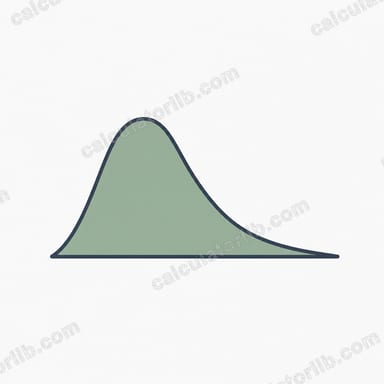
The hybrid lognormal distribution, written HybLogN(\(\rho x, \mu, \sigma\)), is a probability distribution in which the transformed variable \(y(x) = \rho x + \ln(\rho x)\) is normally distributed with mean \(\mu\) and standard deviation \(\sigma\). It blends a normal-distribution term (\(\rho x\)) with a lognormal-distribution term (\(\ln(\rho x)\)). The strength parameter \(\rho > 0\) scales the underlying variable. Because of the logarithm, the distribution is defined only for \(x > 0\). This is a universal piece of pure mathematics and applies identically everywhere.
How to use this calculator
Pick which function to tabulate — the probability density f, the lower cumulative probability P, or the upper cumulative probability Q. Enter the strength parameter \(\rho\), the mean \(\mu\), and the standard deviation \(\sigma\). Then set the initial x, the step size, and the number of rows. The tool evaluates the chosen function at \(x = x_0,\ x_0 + \text{step},\ x_0 + 2\cdot\text{step}, \ldots\) and lists every (x, value) pair, plus the median \(x_c\).
The formula explained
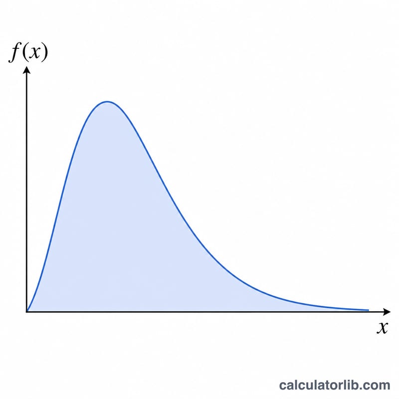
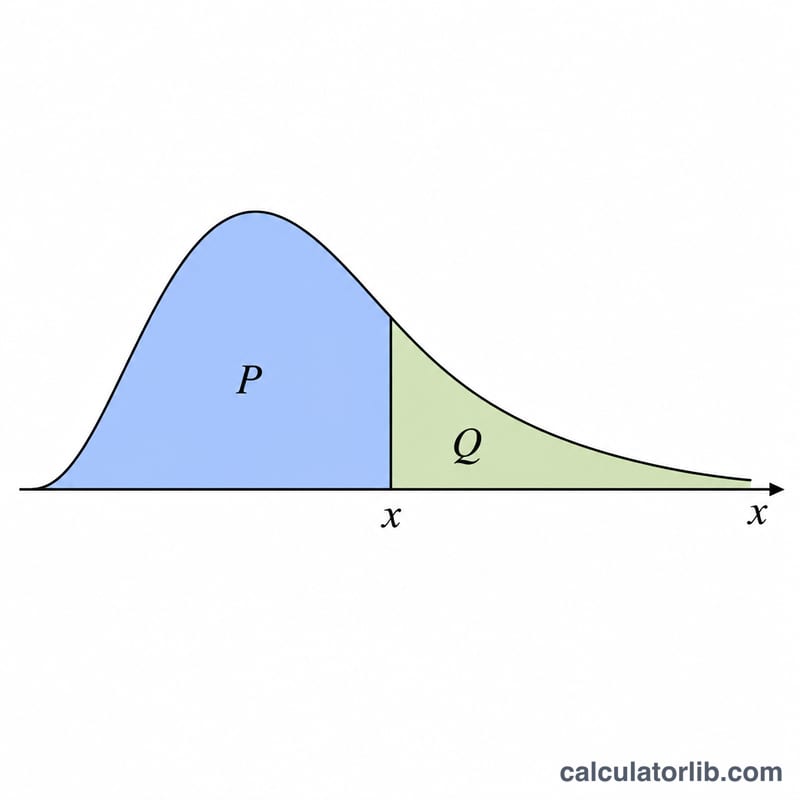
Let \(y(x) = \rho x + \ln(\rho x)\) and \(z = (y(x) - \mu) / \sigma\). The density is $$f(x) = \frac{\rho}{\sqrt{2\pi}\,\sigma}\left(1 + \frac{1}{\rho x}\right) e^{-\frac{1}{2} z^{2}}$$ The factor \(\left(1 + \frac{1}{\rho x}\right)\) is the Jacobian \(dy/dx\) divided by \(\rho\). Since y increases strictly with x and runs from \(-\infty\) to \(+\infty\), the lower cumulative probability is simply \(P(x) = \Phi(z)\), where \(\Phi\) is the standard normal CDF, $$\Phi(z) = \frac{1}{2}\left[1 + \operatorname{erf}\!\left(\frac{z}{\sqrt{2}}\right)\right]$$ The upper cumulative is \(Q(x) = 1 - P(x) = \Phi(-z)\).
Worked example
With \(\rho=1,\ \mu=0,\ \sigma=1\) at \(x=1\): \(y = 1 + \ln(1) = 1\), so \(z = 1\). Density $$f = 0.3989423 \cdot (1+1) \cdot e^{-0.5} = 0.3989423 \cdot 2 \cdot 0.6065307 \approx 0.4839$$ The lower cumulative \(P = \Phi(1) \approx 0.8413\), and the upper cumulative \(Q \approx 0.1587\).
FAQ
Why must x be positive? The term \(\ln(\rho x)\) is undefined for \(\rho x \le 0\). At \(x = 0\) the density is taken as 0, with \(P = 0\) and \(Q = 1\) as limit values.
What is the median? The median \(x_c\) solves \(\rho x_c + \ln(\rho x_c) = \mu\). We solve numerically for \(\rho x_c\) and divide by \(\rho\).
How accurate is the cumulative probability? \(\Phi\) uses the Abramowitz-Stegun 7.1.26 erf approximation, accurate to roughly \(1.5 \times 10^{-7}\).


