What this calculator does
This tool computes the percentage point (also called the quantile or inverse cumulative distribution function) of a Gamma distribution. Given a probability and the Gamma parameters, it returns the value x at which the Gamma cumulative distribution function (CDF) equals that probability. It is the inverse of the Gamma CDF and is widely used in reliability engineering, Bayesian statistics, queueing theory, and rainfall / hydrology modeling.
How to use it
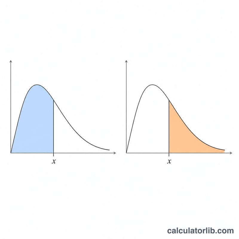
Choose whether your probability is a lower cumulative probability P (area to the left of x) or an upper cumulative probability Q (area to the right). Enter the probability strictly between 0 and 1, the shape parameter a (alpha, must be greater than 0), and the scale parameter b (theta, must be greater than 0). The Gamma mean is a times b. If you use an upper probability Q, the calculator first converts it to \(P = 1 - Q\) before inverting.
The formula explained
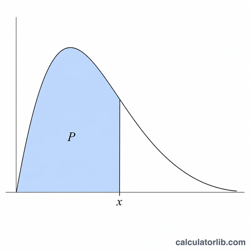
The Gamma CDF in the scale parameterization is $$F(x) = P_{\text{reg}}\!\left(a,\ \frac{x}{b}\right)$$ where \(P_{\text{reg}}\) is the regularized lower incomplete gamma function. Setting \(y = \frac{x}{b}\) makes the problem scale-free: solve \(P_{\text{reg}}(a, y) = P\), then return \(x = b \cdot y\). The regularized incomplete gamma is evaluated with a series expansion for small \(y\) and a continued fraction for large \(y\), and the inversion uses a Wilson-Hilferty initial guess refined by Newton's method, with bisection as a safety fallback.
Worked example
Take probability type = lower, probability = 0.95, shape a = 2, scale b = 1. For \(a = 2\) the CDF has the closed form \(1 - (1 + y)e^{-y}\). Solving $$1 - (1 + y)e^{-y} = 0.95$$ gives \(y \approx 4.7439\), so \(x \approx 4.7439\). With scale \(b = 3\) instead, $$x = 3 \times 4.7439 = 14.2317$$
FAQ
What if a = 1? The Gamma reduces to the Exponential distribution with mean b, and the quantile is the exact closed form $$x = -b \cdot \ln(1 - P)$$
What parameterization is used? Shape a and scale b, so the mean is a times b. If you have a rate parameter, \(b = \frac{1}{\text{rate}}\).
Why must the probability be between 0 and 1? At exactly 0 the quantile is 0 and at exactly 1 it is infinite, so only the open interval \((0, 1)\) returns a finite result.


