What this calculator does
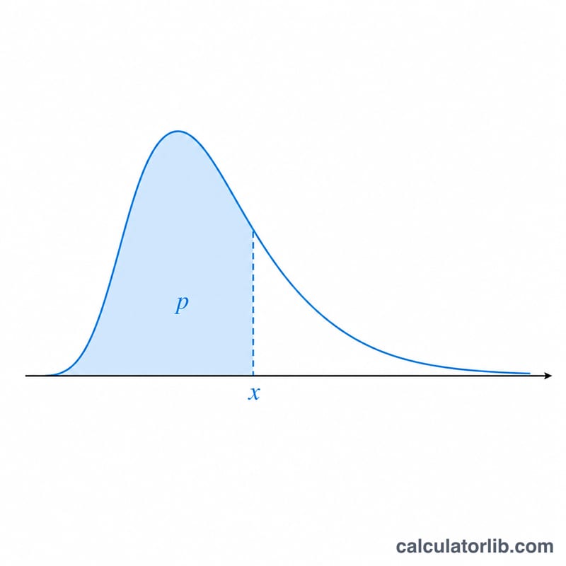
This tool computes the percentile point (quantile) of a lognormal distribution. Given a cumulative probability and the distribution's parameters, it returns the value x at which the lognormal cumulative distribution function (CDF) reaches that probability. It is the inverse CDF, sometimes called the quantile function. The lognormal distribution is widely used for quantities that are positive and right-skewed, such as incomes, particle sizes, stock prices, reliability lifetimes and biological concentrations. This is a universal mathematical tool and applies identically everywhere.
How to use it
Choose whether your probability is a lower-tail value P(X ≤ x) or an upper-tail value P(X > x). Enter the probability (strictly between 0 and 1). Then enter the two parameters of the underlying normal distribution of ln(X): the location parameter mu (the mean of ln X) and the scale parameter sigma (the standard deviation of ln X, which must be positive). Press calculate to get the percentile point x.
The formula explained
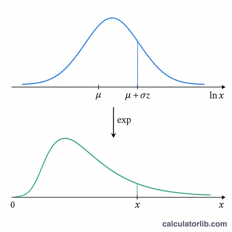
A variable X is lognormal when ln(X) follows a normal distribution with mean mu and standard deviation sigma. Its lower CDF is \( P(x) = \Phi\!\left( \frac{\ln x - \mu}{\sigma} \right) \), where \( \Phi \) is the standard normal CDF. Inverting gives $$ x = \exp\!\left( \mu + \sigma \cdot \Phi^{-1}(p) \right) $$ If you supply an upper-tail probability Q, we first convert it with \( p = 1 - Q \). The standard normal quantile \( \Phi^{-1} \) is evaluated with Acklam's rational approximation, accurate to about 1e-9. Note that mu and sigma describe ln X, not X itself; the mean of X is \( \exp(\mu + \sigma^{2}/2) \).
Worked example
Take lower mode, probability = 0.975, mu = 0, sigma = 1. Then \( p = 0.975 \) and \( \Phi^{-1}(0.975) = 1.959964 \) (the classic 1.96 critical value). So $$ x = \exp(0 + 1 \times 1.959964) = 7.0994 $$ The 97.5th percentile of the standard lognormal is about 7.099.
FAQ
What if I use upper mode? Entering Q = 0.025 in upper mode gives \( p = 1 - 0.025 = 0.975 \) and the same \( x \approx 7.099 \) as the example above.
What is the median? For \( p = 0.5 \), \( \Phi^{-1}(0.5) = 0 \), so \( x = \exp(\mu) \). The median of a lognormal distribution is \( \exp(\mu) \) regardless of sigma.
Why must 0 < p < 1? As p approaches 0 the percentile approaches 0, and as p approaches 1 it diverges to infinity, so endpoints are rejected. The result is always positive because it is an exponential.


