
What this calculator does
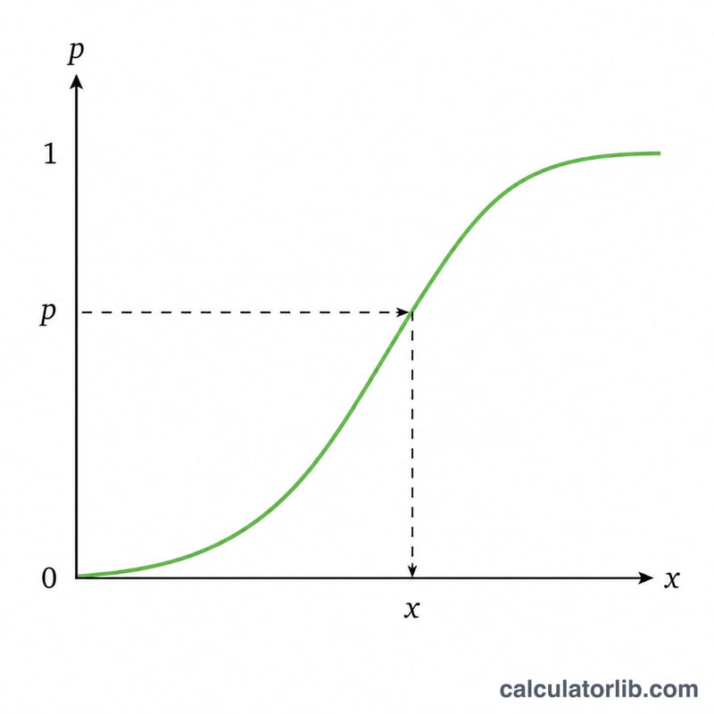
The logistic distribution is a continuous probability distribution shaped like a normal curve but with heavier tails. It is widely used in logistic regression, growth modeling, and reliability analysis. This tool solves the inverse problem: given a cumulative probability, it returns the percentile point x (also called the quantile) where the logistic cumulative distribution function (CDF) reaches that probability.
How to use it
Choose whether your probability is a lower cumulative value P(X ≤ x) or an upper cumulative value P(X > x). Enter the probability as a number strictly between 0 and 1, then provide the location parameter a (the mean and median) and the scale parameter b, which must be greater than 0. The calculator returns x along with the lower-tail probability actually used and its logit (log-odds).
The formula explained
The logistic CDF is \(F(x) = 1 / (1 + e^{-(x-a)/b})\). Solving for x gives the quantile function:
$$x = \text{a} + \text{b} \cdot \ln\!\left(\frac{\text{p}}{1 - \text{p}}\right)$$Here p is the lower-tail probability. If you supplied an upper-tail value Q, the calculator first converts it with \(p = 1 - Q\). The term \(\ln(p / (1 - p))\) is the logit, or log-odds, of the probability. When \(p = 0.5\) the logit is 0, so the quantile equals the location a, confirming that a is the median.
Worked example
Suppose probabilityType = lower, probability = 0.9, a = 5, b = 2. Then \(p / (1 - p) = 0.9 / 0.1 = 9\), and \(\ln(9) = 2.197224577\). So $$x = 5 + 2 \times 2.197224577 = 9.394449.$$ The 90th percentile of this logistic distribution is about 9.39.
FAQ
What happens at probability 0.5? The quantile is exactly the location a, because the logistic distribution is symmetric about its mean and median.
Why must the probability be strictly between 0 and 1? As the probability approaches 0 the quantile tends to negative infinity, and as it approaches 1 it tends to positive infinity, so the endpoints have no finite value.
What is the scale parameter b? It controls the spread of the distribution; larger b stretches the curve. The standard deviation equals \(b\pi/\sqrt{3}\).


