這個計算器的功能
羅吉斯分布(Logistic distribution)是一種連續型機率分布,外形類似常態分布的鐘形曲線,但尾部更厚。它廣泛應用於羅吉斯迴歸、成長模型與可靠度分析。本工具解決的是反向問題:給定一個累積機率,回傳羅吉斯累積分布函數(CDF)達到該機率時所對應的百分位數點 \(x\)(也稱為分位數)。
使用方式
首先選擇你的機率屬於下尾累積值 \(P(X \le x)\),還是上尾累積值 \(P(X > x)\)。接著輸入一個嚴格介於 0 與 1 之間的機率數值,再填入位置參數 \(a\)(即平均數與中位數)以及尺度參數 \(b\)(必須大於 0)。計算器會回傳 \(x\),並同時顯示實際使用的下尾機率及其 logit(對數勝算比)。
公式說明
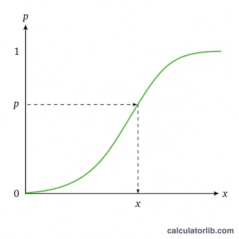
羅吉斯分布的 CDF 為 \(F(x) = 1 / (1 + e^{-(x-a)/b})\)。對 \(x\) 求解後可得分位數函數:
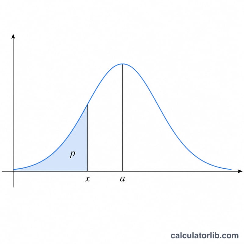
$$x = \text{a} + \text{b} \cdot \ln\!\left(\frac{\text{p}}{1 - \text{p}}\right)$$其中 \(p\) 為下尾機率。若你輸入的是上尾值 \(Q\),計算器會先以 \(p = 1 - Q\) 進行換算。式中的 \(\ln(p / (1 - p))\) 就是該機率的 logit,也就是對數勝算比。當 \(p = 0.5\) 時,logit 為 0,因此分位數會等於位置參數 \(a\),這也印證了 \(a\) 即為中位數。
範例演算
假設 probabilityType = 下尾、probability = 0.9、a = 5、b = 2。則 \(p / (1 - p) = 0.9 / 0.1 = 9\),而 \(\ln(9) = 2.197224577\)。所以 $$x = 5 + 2 \times 2.197224577 = 9.394449$$也就是說,此羅吉斯分布的第 90 百分位數約為 9.39。
常見問題
當機率為 0.5 時會發生什麼?此時分位數恰好等於位置參數 \(a\),因為羅吉斯分布以其平均數與中位數為中心呈對稱分布。
為什麼機率必須嚴格介於 0 與 1 之間?當機率趨近 0 時,分位數會趨向負無限大;趨近 1 時,則趨向正無限大,因此兩端點都沒有有限的數值。
尺度參數 \(b\) 是什麼?它控制分布的離散程度;\(b\) 越大,曲線就越被拉寬。其標準差等於 \(b\pi/\sqrt{3}\)。