
What is the logistic distribution?
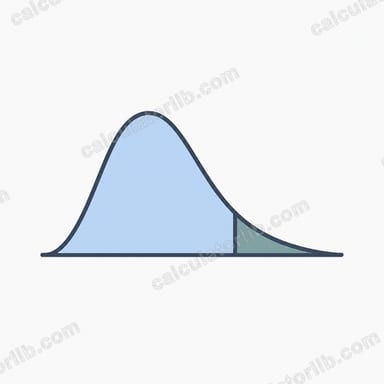
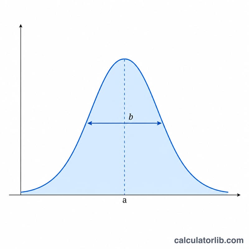
The logistic distribution is a continuous probability distribution shaped like the normal distribution but with heavier tails. It is defined by a location parameter a (which equals its mean and median) and a scale parameter b > 0. Its cumulative distribution function is the familiar logistic sigmoid, which is why the distribution appears throughout logistic regression, growth modeling, and machine learning. This calculator is pure mathematics and applies identically everywhere, with no country-specific assumptions.
How to use this calculator
Pick which function to compute: probability density f, lower cumulative probability P (the CDF), or upper cumulative probability Q (the survival function). Enter the location a and scale b. Then describe the x grid: the initial x, the step, and the number of points. The tool generates \(x_i = \text{startX} + i\cdot\text{stepX}\) for \(i = 0..\text{points}-1\), evaluates the chosen function at each, shows the headline value at the first x, lists the series, and draws a line graph.
The formula explained
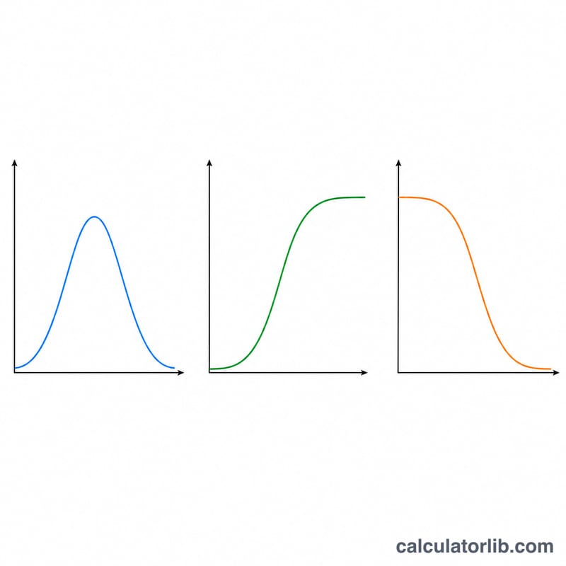
Define the standardized variable \(z = (x - a)/b\) and \(E = e^{-z}\). The density is $$f = \frac{1}{b}\cdot\frac{E}{(1+E)^2}.$$ Writing the sigmoid \(\sigma = 1/(1+E)\), this equals \(\sigma(1-\sigma)/b\). The lower CDF is simply $$P = \sigma = \frac{1}{1+e^{-z}},$$ increasing monotonically from 0 to 1, and the upper (survival) function is \(Q = 1 - P\). To avoid overflow, the sigmoid is computed as \(1/(1+e^{-z})\) when \(z \geq 0\) and \(e^z/(1+e^z)\) when \(z < 0\).
Worked example
With \(a = 0\) and \(b = 0.7\), evaluate at \(x = 0.7\). Then \(z = 1\) and \(E = e^{-1} = 0.367879\). Density $$f = \frac{1}{0.7}\cdot\frac{0.367879}{(1.367879)^2} \approx 0.28087.$$ Lower CDF $$P = \frac{1}{1.367879} \approx 0.73106.$$ Upper CDF $$Q = 1 - 0.73106 \approx 0.26894.$$ At the median \(x = a = 0\) you get the peak density \(1/(4b) = 0.35714\) and \(P = Q = 0.5\).
FAQ
What if b is zero or negative? The distribution is undefined; the calculator requires \(b > 0\) and returns an error otherwise.
What are the mean and variance? The mean (and median) equals \(a\), and the variance is \((\pi^2/3)\cdot b^2\).
Can I use a descending grid? Yes — a negative step produces x values that decrease, and a step of 0 evaluates every point at the initial x.