
What is the geometric distribution?
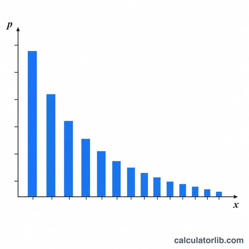
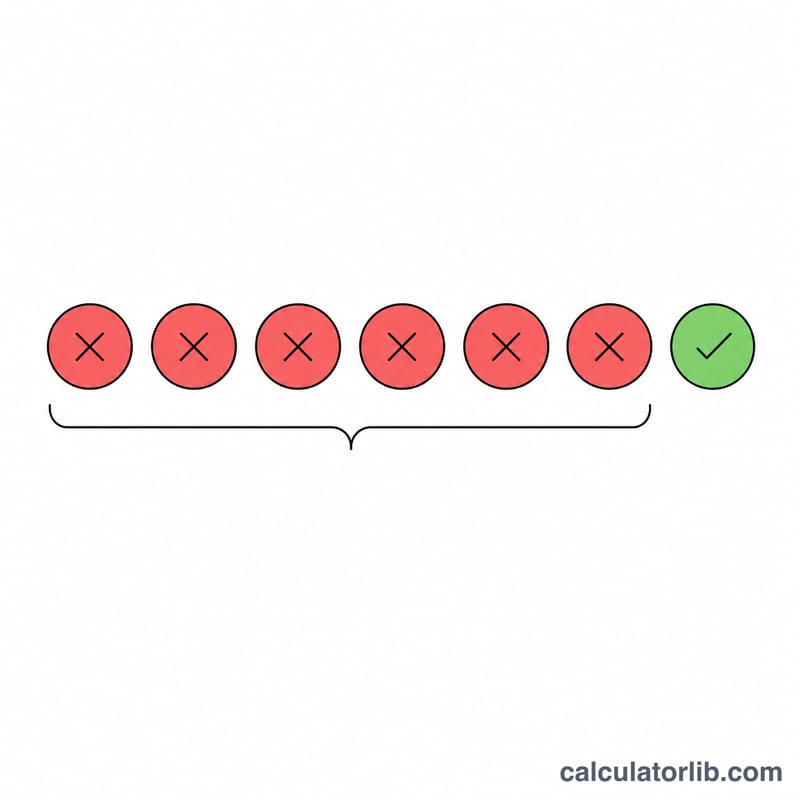
The geometric distribution models the number of failures that occur before the first success in a sequence of independent trials, each with the same success probability p. This calculator uses the "number of failures before the first success" convention, so the random variable x takes values 0, 1, 2, ... and the probability mass function is \(f(x,p) = p(1-p)^{x}\). Note: a different common form counts the trial number k of the first success (k = 1, 2, ...); that is not the one used here, where \(x = k - 1\).
How to use this calculator
Enter the number of failures before the first success x (a non-negative integer) and the per-trial success probability p (a value between 0 and 1). The tool returns the probability mass \(f(x,p)\), the lower cumulative probability \(P(X \le x)\), the upper cumulative probability \(P(X \ge x)\), and the mean (expected number of failures).
The formulas explained
Let \(q = 1 - p\). The probability mass is $$f(x,p) = p\cdot q^{x}.$$ The lower cumulative sum telescopes to $$P(X \le x) = 1 - q^{x+1}.$$ The upper tail is $$P(X \ge x) = q^{x}.$$ The mean is $$E[X] = \frac{1 - p}{p}.$$ A useful identity is \(P(X \le x) + P(X \ge x) = 1 + f(x,p)\), because the two tails both count the point x.
Worked example
With x = 2 and p = 0.4 (so q = 0.6): $$f(2, 0.4) = 0.4 \cdot 0.6^{2} = 0.4 \cdot 0.36 = 0.144.$$ Lower cumulative $$P(X \le 2) = 1 - 0.6^{3} = 1 - 0.216 = 0.784.$$ Upper cumulative $$P(X \ge 2) = 0.6^{2} = 0.36.$$ Mean \(= 0.6/0.4 = 1.5\). Check: \(0.784 + 0.36 - 0.144 = 1.000\).
FAQ
Does x count the successful trial? No. Here x counts only the failures before the first success, so x starts at 0. If you have the trial number k of the first success, use \(x = k - 1\).
What happens when p = 1? Success is guaranteed on the first trial: \(f(0,1) = 1\), \(f(x,1) = 0\) for \(x \ge 1\), and the mean is 0.
Why is the mean undefined when p = 0? If no trial ever succeeds, the expected number of failures is infinite, so the formula \((1 - p)/p\) divides by zero.


