What is the inverse chi-squared distribution?
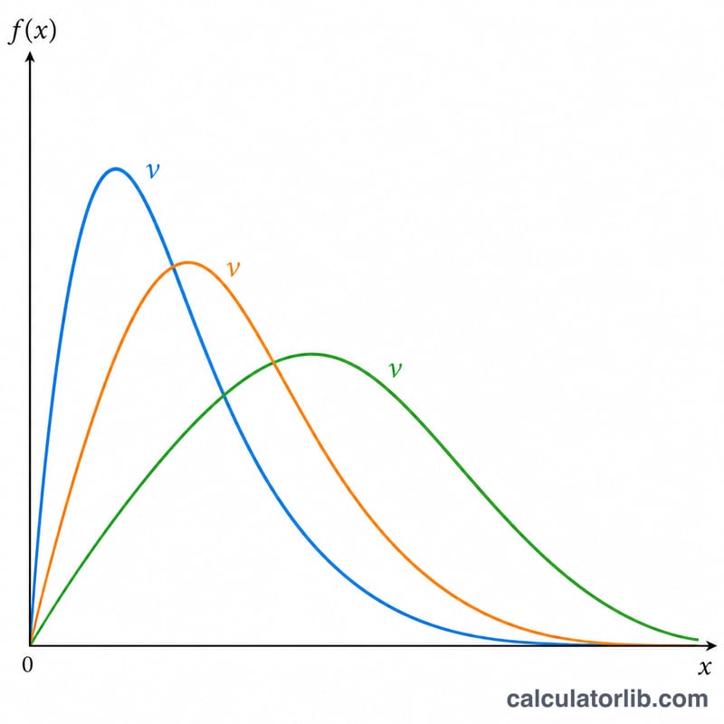
The inverse chi-squared distribution with ν (nu) degrees of freedom is the distribution of \(Y = 1/X\), where X follows a standard chi-squared distribution with ν degrees of freedom. It is widely used in Bayesian statistics as a conjugate prior for the variance of a normal distribution, and it appears in reliability and signal-processing models. This calculator is pure mathematics, so it applies identically everywhere with no regional rules.
How to use this calculator
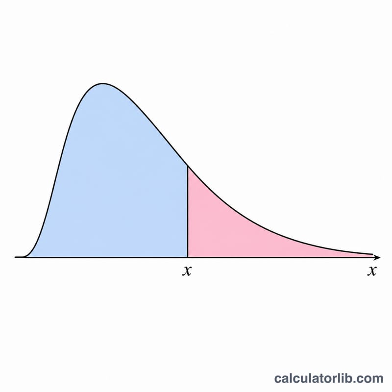
Enter the percentile point x (any positive real number) and the degrees of freedom ν (any positive value; usually a positive integer). The tool returns three quantities: the probability density \(f(x)\), the lower cumulative probability \(P = P(X \le x)\), and the upper cumulative probability \(Q = P(X > x)\). Because P and Q describe the whole distribution, they always sum to 1.
The formula explained
The density is $$f(x) = \frac{2^{-\nu/2}}{\Gamma\!\left(\frac{\nu}{2}\right)}\, x^{-\frac{\nu}{2}-1}\, e^{-\frac{1}{2x}}$$ for \(x > 0\). For numerical stability we compute it in log space using the log-gamma function. The cumulative probabilities use the reciprocal link to the chi-squared distribution: with \(s = \nu/2\) and \(z = 1/(2x)\), the lower cumulative probability equals the regularized upper incomplete gamma \(Q(s, z)\), and the upper cumulative probability equals the regularized lower incomplete gamma \(P(s, z)\). These are evaluated with a series expansion for small z and a continued-fraction (Lentz) method for large z.
Worked example
Take \(x = 1\) and \(\nu = 1\). Then \(s = 0.5\) and \(z = 0.5\). The density evaluates to \(f(1) \approx 0.241971\). The lower cumulative probability is \(P \approx 0.317311\) and the upper cumulative probability is \(Q \approx 0.682689\), which correctly sum to 1.
FAQ
Why must x be greater than 0? The support of the distribution is \(x > 0\). For \(x \le 0\) the density is 0; all probability mass lies above, so the lower probability is 0 and the upper is 1.
Does ν have to be an integer? No. The formula uses the gamma function, so any real \(\nu > 0\) works, though degrees of freedom are most often positive integers.
Is this the scaled inverse chi-squared? No. This is the standard (non-scaled) inverse chi-squared distribution, matching the reciprocal of a chi-squared variable.


