What this calculator does
This tool computes the percentage point (also called the quantile, critical value, or inverse CDF) of Student's t-distribution. Given a cumulative probability P and the degrees of freedom nu, it returns the value t for which the area under the t density up to t equals the chosen probability. It is the inverse of the t-distribution cumulative distribution function and corresponds to the t.inv spreadsheet function. The t-distribution is universal pure mathematics and applies identically everywhere.
How to use it
Enter the cumulative probability P (strictly between 0 and 1), choose whether P is a lower-tail area (to the left of t) or an upper-tail area (to the right of t), and enter the degrees of freedom. Internally the calculator always converts to a lower-tail probability: for a lower tail it uses P directly, and for an upper tail it uses 1 - P. It then solves for t.
The formula explained
The CDF of Student's t with nu degrees of freedom is written with the regularized incomplete beta function I. For \(t \ge 0\), \(F(t) = 1 - \tfrac{1}{2}\,I_x(\tfrac{\nu}{2}, \tfrac{1}{2})\) with \(x = \frac{\nu}{\nu + t^2}\); for \(t < 0\) the symmetric expression \(F(t) = \tfrac{1}{2}\,I_x(\tfrac{\nu}{2}, \tfrac{1}{2})\) is used. The incomplete beta is evaluated with the Lanczos approximation for the gamma function and the standard continued-fraction algorithm. Because F is strictly increasing, the inverse is found by robust bisection.
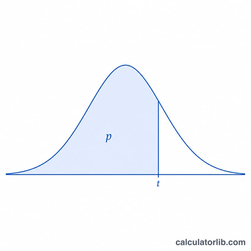
The percentage point is the inverse CDF:
$$t = F^{-1}\!\left(\text{P};\ \nu\right)$$Equivalently, for a lower-tail probability:
$$F(t) = \text{P} \quad\Longrightarrow\quad t = F^{-1}\!\left(\text{P}\right)$$and for an upper-tail probability:
$$F(t) = 1-\text{P} \quad\Longrightarrow\quad t = F^{-1}\!\left(1-\text{P}\right)$$where
$$F(t)=1-\tfrac{1}{2}\,I_{x}\!\left(\tfrac{\nu}{2},\tfrac{1}{2}\right),\quad x=\frac{\nu}{\nu+t^{2}},\quad \nu=\text{df}$$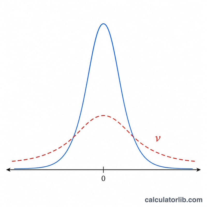
Worked example
For \(P = 0.975\), lower tail, and \(\nu = 10\) degrees of freedom, the calculator returns
$$t \approx 2.228139$$— the familiar two-sided 95% (one-sided 97.5%) critical value found in t-tables. The same answer arises from \(P = 0.025\) with the upper tail, since an upper 2.5% area equals a lower 97.5% area.
FAQ
What if I enter P = 0 or P = 1? The percentage point is undefined; it diverges to minus or plus infinity, so the calculator reports an error.
What happens as the degrees of freedom grow large? The t-distribution approaches the standard normal, so for very large nu the quantile approaches the normal quantile (e.g. \(P = 0.975\) gives about \(1.95996\)).
Can nu be a non-integer? Yes. Any \(\nu > 0\) is accepted, including fractional values.


